For many enterprises, critical business information is often stored as unstructured data scattered across multiple content repositories. Not only is it challenging for organizations to make this information available to employees when they need it, but it’s also difficult to do so securely so relevant information is available to the right employees or employee groups.
Amazon Kendra is a highly accurate and easy-to-use intelligent search service powered by machine learning (ML). Amazon Kendra delivers secure search for enterprise applications and can make sure the results of a user’s search query only include documents the user is authorized to read. In this post, we illustrate how to build an Amazon Kendra-powered search application supporting access controls that reflect the security model of an example organization.
Amazon Kendra supports search filtering based on user access tokens that are provided by your search application, as well as document access control lists (ACLs) collected by the Amazon Kendra connectors. When user access tokens are applied, search results return links to the original document repositories and include a short description. Access control to the full document is still enforced by the original repository.
In this post, we demonstrate token-based user access control in Amazon Kendra with Open ID. We use Amazon Cognito user pools to authenticate users and provide Open ID tokens. You can use a similar approach with other Open ID providers.
Application overview
This application is designed for guests and registered users to make search queries to a document repository, and results are returned only from those documents that are authorized for access by the user. Users are grouped based on their roles, and access control is at a group level. The following table outlines which documents each user is authorized to access for our use case. The documents being used in this example are a subset of AWS public documents.
| User | Role | Group | Document Type Authorized for Access |
| Guest | Blogs | ||
| Patricia | IT Architect | Customer | Blogs, user guides |
| James | Sales Rep | Sales | Blogs, user guides, case studies |
| John | Marketing Exec | Marketing | Blogs, user guides, case studies, analyst reports |
| Mary | Solutions Architect | Solutions Architect | Blogs, user guides, case studies, analyst reports, whitepapers |
Architecture
The following diagram illustrates our solution architecture.

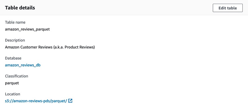
The documents being queried are stored in an Amazon Simple Storage Service (Amazon S3) bucket. Each document type has a separate folder: blogs, case-studies, analyst-reports, user-guides, and white-papers. This folder structure is contained in a folder named Data. Metadata files including the ACLs are included in a folder named Meta.
We use the Amazon Kendra S3 connector to configure this S3 bucket as the data source. When the data source is synced with the Amazon Kendra index, it crawls and indexes all documents as well as collects the ACLs and document attributes from the metadata files. For this example, we use a custom attribute DocumentType to denote the type of the document.
We use an Amazon Cognito user pool to authenticate registered users, and use an identity pool to authorize the application to use Amazon Kendra and Amazon S3. The user pool is configured as an Open ID provider in the Amazon Kendra index by configuring the signing URL of the user pool.
When a registered user authenticates and logs in to the application to perform a query, the application sends the user’s access token provided by the user pool to the Amazon Kendra index as a parameter in the query API call. For guest users, there is no authentication and therefore no access token is sent as a parameter to the query API. The results of a query API call without the access token parameter only return the documents without access control restrictions.
When an Amazon Kendra index receives a query API call with a user access token, it decrypts the access token using the user pool signing URL and gets parameters such as cognito:username and cognito:groups associated with the user. The Amazon Kendra index filters the search results based on the stored ACLs and the information received in the user access token. These filtered results are returned in response to the query API call made by the application.
The application, which the users can download with its source, is written in ReactJS using components from the AWS Amplify framework. We use the AWS Amplify console to implement the continuous integration and continuous deployment pipelines. We use an AWS CloudFormation template to deploy the AWS infrastructure, which includes the following:
- An Amazon Kendra index
- An Amazon Cognito user pool and identity pool
- AWS Identity and Access Management (IAM) roles and policies
- An AWS CodeCommit source code repository
- AWS Amplify console application configurations
In this post, we provide a step-by-step walkthrough to configure the backend infrastructure, build and deploy the application code, and use the application.
Prerequisites
To complete the steps in this post, make sure you have the following:
- An AWS account with privileges to create IAM roles and policies.
- Basic knowledge of AWS.
- An S3 bucket for your documents. For more information, see Creating a bucket and What is Amazon S3?
- Access to a command terminal with the AWS Command Line Interface (CLI) installed or AWS CloudShell. For instructions, see Installing, updating, and uninstalling the AWS CLI version 2.
- Amazon Kendra.
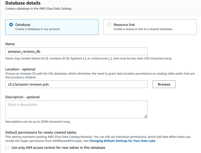
Preparing your S3 bucket as a data source
To prepare an S3 bucket as a data source, create an S3 bucket. In the terminal with the AWS CLI or AWS CloudShell, run the following commands to upload the documents and the metadata to the data source bucket:
aws s3 cp s3://aws-ml-blog/artifacts/building-a-secure-search-application-with-access-controls-kendra/docs.zip .
unzip docs.zip
aws s3 cp Data/ s3://<REPLACE-WITH-NAME-OF-S3-BUCKET>/Data/ --recursive
aws s3 cp Meta/ s3://<REPLACE-WITH-NAME-OF-S3-BUCKET>/Meta/ --recursive
Deploying the infrastructure as a CloudFormation stack
In a separate browser tab open the AWS Management Console, and make sure that you are logged in to your AWS account. Click the button below to launch the CloudFormation stack to deploy the infrastructure.
![]()
You should see a page similar to the image below:

For S3DataSourceBucket, enter your data source bucket name without the s3:// prefix, select I acknowledge that AWS CloudFormation might create IAM resources with custom names, and then choose Create stack.
Stack creation can take 30–45 minutes to complete. While you wait, you can look at the different tabs, such as Events, Resources, and Template. You can monitor the stack creation status on the Stack info tab.

When stack creation is complete, keep the Outputs tab open. We need values from the Outputs and Resources tabs in subsequent steps.
Reviewing Amazon Kendra configuration and starting the data source sync
In the following steps, we configure Amazon Kendra to enable secure token access and start the data source sync to begin crawling and indexing documents.
- On the Amazon Kendra console, choose the index
AuthKendraIndex, which was created as part of theCloudFormationstack.

Under User access control, token-based user access control is enabled, the signing key object is set to the Open ID provider URL of the Amazon Cognito user pool, and the user name and group are set to cognito:username and cognito:groups, respectively.

- In the navigation pane, choose Data sources.
- On the Settings tab, you can see the data source bucket being configured.
- Select the radio button for the data source and choose Sync now.

The data source sync can take 10–15 minutes to complete, but you don’t have to wait to move to the next step.
Creating users and groups in the Amazon Cognito user pool
In the terminal with the AWS CLI or AWS CloudShell, run the following commands to create users and groups in the Amazon Cognito user pool to use for our application. You need to copy the contents of the Physical ID column in the UserPool row from the Resources tab of the CloudFormation stack. This is the user pool ID to use in the following steps. We set AmazonKendra@2020 as the temporary password for all the users. This password is required when logging in for the first time, and Amazon Cognito enforces a password reset.
USER_POOL_ID=<PASTE-USER-POOL-ID-HERE>
aws cognito-idp create-group --group-name customer --user-pool-id ${USER_POOL_ID}
aws cognito-idp create-group --group-name AWS-Sales --user-pool-id ${USER_POOL_ID}
aws cognito-idp create-group --group-name AWS-Marketing --user-pool-id ${USER_POOL_ID}
aws cognito-idp create-group --group-name AWS-SA --user-pool-id ${USER_POOL_ID}
aws cognito-idp admin-create-user --user-pool-id ${USER_POOL_ID} --username patricia --temporary-password AmazonKendra@2020
aws cognito-idp admin-create-user --user-pool-id ${USER_POOL_ID} --username james  --temporary-password AmazonKendra@2020
aws cognito-idp admin-create-user --user-pool-id ${USER_POOL_ID} --username john  --temporary-password AmazonKendra@2020
aws cognito-idp admin-create-user --user-pool-id ${USER_POOL_ID} --username mary  --temporary-password AmazonKendra@2020
aws cognito-idp admin-add-user-to-group --user-pool-id ${USER_POOL_ID} --username patricia --group-name customer
aws cognito-idp admin-add-user-to-group --user-pool-id ${USER_POOL_ID} --username james --group-name AWS-Sales
aws cognito-idp admin-add-user-to-group --user-pool-id ${USER_POOL_ID} --username john --group-name AWS-Marketing
aws cognito-idp admin-add-user-to-group --user-pool-id ${USER_POOL_ID} --username mary --group-name AWS-SA
Building and deploying the app
Now we build and deploy the app using the following steps:
- On the AWS Amplify console, choose the app
AWSKendraAuthApp. - Choose Run build.

You can monitor the build progress on the console.

Let the build continue and complete the steps: Provision, Build, Deploy, and Verify. After this, the application is deployed and ready to use.
You can browse through the source code by opening up the CodeCommit repository. The important file to look at is src/App.tsx.
- Choose the link on the left to start the application in a new browser tab.

Trial run
We can now take a trial run of our app.
- On the login page, sign in with the username
patriciaand the temporary passwordAmazonKendra@2020.

Amazon Cognito requires you to reset your password the first time you log in. After you log in, you can see the search field.

- In the search field, enter a query, such as
what is serverless? - Expand Filter search results to see different document types.
You can select different document types to filter the search results.
- Sign out and repeat this process for other users that are created in the Cognito user pool, namely,
james,john, andmary.
You can also choose Continue as Guest to use the app without authenticating. However, this option only shows results from blogs.

You can return back to the login screen by choosing Welcome Guest! Click here to sign up or sign in.
Using the application
You can use the application we developed by making a few search queries logged in as different users. To experience how access control works, issue the same query from different user accounts and observe the difference in the search results. The following users get results from different sources:
- Guests and anonymous users – Only blogs
- Patricia (Customer) – Blogs and user guides
- James (Sales) – Blogs, user guides, and case studies
- John (Marketing) – Blogs, user guides, case studies, and analyst reports
- Mary (Solutions Architect) – Blogs, user guides, case studies, analyst reports, and whitepapers
We can make additional queries and observe the results. Some suggested queries include “What is machine learning?”, “What is serverless?”, and “Databases”.
Cleaning up
To delete the infrastructure that was deployed as part of the CloudFormation stack, delete the stack from the AWS CloudFormation console. Stack deletion can take 20–30 minutes.
When the stack status shows as Delete Complete, go to the Events tab and confirm that each of the resources has been removed. You can also cross-verify by checking on the respective management consoles for Amazon Kendra, Amazon Amplify, and the Amazon Cognito user pool and identity pool.
You must delete your data source bucket separately, because it was not created as part of the CloudFormation stack.
Conclusion
In this post, we demonstrated how you can create a secure search application using Amazon Kendra. Organizations who use an Open ID-compliant identity management system with a new or pre-existing Amazon Kendra index can now enable secure token access to make sure your intelligent search applications are aligned with your organizational security model. For more information about access control in Amazon Kendra, see Controlling access to documents in an index.
About the Author
 Abhinav Jawadekar is a Senior Partner Solutions Architect at Amazon Web Services. Abhinav works with AWS partners to help them in their cloud journey.


 Yunzhi Shi is a data scientist at the Amazon ML Solutions Lab where he helps AWS customers address business problems with AI and cloud capabilities. Recently, he has been building computer vision, search, and forecast solutions for various customers.


 Talia Chopra is a Technical Writer in AWS specializing in machine learning and artificial intelligence. She works with multiple teams in AWS to create technical documentation and tutorials for customers using Amazon SageMaker, MxNet, and AutoGluon.
 Phil Cunliffe is an engineer turned Software Development Manager for Amazon Human in the Loop services. He is a JavaScript fanboy with an obsession for creating great user experiences.

 Azim Siddique serves as Technical Advisor and CoE Architect at Foxconn. He provides architectural direction for the Digital Transformation program, conducts PoCs with emerging technologies, and guides engineering teams to deliver business value by leveraging digital technologies at scale.
 Felice Chuang is a Data Architect at Foxconn. She uses her diverse skillset to implement end-to-end architecture and design for big data, data governance, and business intelligence applications. She supports analytic workloads and conducts PoCs for Digital Transformation programs.
 Yash Shah is a data scientist in the Amazon ML Solutions Lab, where he works on a range of machine learning use cases from healthcare to manufacturing and retail. He has a formal background in Human Factors and Statistics, and was previously part of the Amazon SCOT team designing products to guide 3P sellers with efficient inventory management.
 Dan Volk is a Data Scientist at Amazon ML Solutions Lab, where he helps AWS customers across various industries accelerate their AI and cloud adoption. Dan has worked in several fields including manufacturing, aerospace, and sports and holds a Masters in Data Science from UC Berkeley.
 Rodrigo Alarcon is a Sr. Solutions Architect with AWS based out of Santiago, Chile. Rodrigo has over 10 years of experience in IT security and network infrastructure. His interests include machine learning and cybersecurity.


 Surya Kari is a Data Scientist who works on AI devices within AWS. His interests lie in computer vision and autonomous systems.


 Mithil Shah is an ML/AI Specialist at Amazon Web Services. Currently he helps public sector customers improve lives of citizens by building Machine Learning solutions on AWS.
 Paul Saxman is a Principal Solutions Architect at AWS, where he helps clinicians, researchers, executives, and staff at academic medical centers to adopt and leverage cloud technologies. As a clinical and biomedical informatics, Paul is passionate about accelerating healthcare advancement and innovation, by supporting the translation of science into medical practice.