Rapid development of deep learning technology has produced an abundance of open-sourced, pre-trained models in computer vision and natural language processing. As a result, transfer learning has become a popular approach in deep learning. Transfer learning is a machine learning technique where a model pre-trained on one task is fine-tuned on a new task. Given the significant compute and time resources required to develop neural network models, adapting a pre-trained model to new data is compelling in business applications. If you’re new to deep learning, transfer learning is also a good starting point because you don’t have to build a model from scratch. For deep learning beginners, one question you may have is, how do I systematically examine model predictions to see what mistakes were made now that my data is in the form of pictures or text?
In this post, we show you an end-to-end example of doing transfer learning by using Amazon SageMaker Debugger to detect hidden problems that may have serious consequences. Debugger doesn’t incur additional costs if you’re running training on Amazon SageMaker. Moreover, you can enable the built-in rules with just a few lines of code when you call the Amazon SageMaker estimator function. For our use case, we do transfer learning using a ResNet model to recognize German traffic signs [1].
In this post, we focus on issues that occur during training. For more information about using Debugger for inference and explainability, see Detecting and analyzing incorrect model predictions with Amazon SageMaker Model Monitor and Debugger.
Setting up a transfer learning training job
For our use case, we want to adapt a pre-trained computer vision model to recognize traffic signs in Germany. We use the GTSRB dataset [1] for this new task. You can find the notebook and training script in the GitHub repo.
Applying preprocessing on the dataset
We first apply some typical preprocessing for a ResNet model on our dataset (see the complete notebook for where to download the dataset). To improve model generalization, we apply data augmentation (RandomResizedCrop and RandomHorizontalFlip). These operations ensure that an image looks differently in each epoch. Lastly, we normalize the data: because the model has been pre-trained on the ImageNet dataset, we apply the same preprocessing and normalization (subtract the mean and divide by the standard deviation of the ImageNet dataset). See the following code:
from torchvision import datasets, models, transforms

# Define pre-processing
train_transform =  transforms.Compose([
                                        transforms.RandomResizedCrop(224),
                                        transforms.RandomHorizontalFlip(),
                                        transforms.ToTensor(),
                                        transforms.Normalize([0.485, 0.456, 0.406], [0.229, 0.224, 0.225])
                                    ])
We use Pytorch’s ImageFolder function, which takes a local folder and loads all images located in the subdirectories and encodes the directory name as a label. Next we specify the dataloader that takes the batch size and dataset. We use the dataloader during training to provide new batches in each iteration. See the following code:
# Apply the pre-processing to the training dataset
dataset = datasets.ImageFolder(root='GTSRB/Training', transform=train_transform)
train_dataloader = torch.utils.data.DataLoader(dataset, batch_size=64, shuffle=True)
For the validation dataset, we don’t apply data augmentation and only resize images to the appropriate size:
# Apply the pre-processing to validation dataset
val_transform = transforms.Compose([
                                        transforms.Resize(256),
                                        transforms.CenterCrop(224),
                                        transforms.ToTensor(),
                                        transforms.Normalize([0.485, 0.456, 0.406], [0.229, 0.224, 0.225])
                                        ])

dataset_test = datasets.ImageFolder(root='GTSRB/Final_Test', transform=val_transform)
val_dataloader = torch.utils.data.DataLoader(dataset, batch_size=64, shuffle=False)
Loading a pre-trained ResNet model
Because we have a limited variety of traffic signs, we pick a simpler ResNet model for this task: resnet18. You can load a ResNet18 from the PyTorch model zoo with pre-trained weights using just one line of code:
#get pretrained ResNet model
model = models.resnet18(pretrained=True)
The model has been pre-trained on the ImageNet dataset, which consists of 1,000 image classes. For our use case, we fine-tune it on a dataset that only has 43 classes. We adjust the last layer, which is a fully connected Linear layer:
#traffic sign dataset has 43 classes
nfeatures = model.fc.in_features
model.fc = torch.nn.Linear(nfeatures, 43)
Because we train a multi-classification model, we use the cross entropy loss function:
#loss for multi label classification
loss_function = torch.nn.CrossEntropyLoss()
Next we specify the optimizer that takes the model parameters and learning rate. Here we use the stochastic gradient descent optimizer:
# optimizer
optimizer = torch.optim.SGD(model.parameters(), lr=0.001)
Defining the training loop
The following code blocks define the training loop. We iterate over ten epochs, perform the forward and backward pass, and update the model parameters.
for epoch in range(10):  # loop over the entire dataset 10 times

    for data in train_dataloader:

        # get the inputs; data is a list of [inputs, labels]
        inputs, labels = data

        # zero the parameter gradients
        optimizer.zero_grad()

        # forward
        outputs = model(inputs)

        #compute loss
        loss = loss_function(outputs, labels)

        #backward pass
        loss.backward()

        #optimize
        optimizer.step()

        #get predictions
        _, preds = torch.max(outputs, 1)

        # statistics
        epoch_loss += loss.item()

        print('Epoch {}/{} Loss: {:.4f}'.format(epoch, 1, epoch_loss))
If you just run the preceding code, the training runs just on your Amazon SageMaker notebook. To make the most out of Amazon SageMaker, you want to use the pre-built DLC containers, which come with optimized performance and let you access the full feature sets of Debugger at no additional cost. By running on Amazon SageMaker, we can easily train our models at scale. Most deep learning models are trained on GPU due to the computational intensity. With Amazon SageMaker, GPU instances are automatically created and torn down after training completes, so you only pay for the time the resources were used.
Making a training script compatible with Amazon SageMaker
To run training on Amazon SageMaker, you need to change the location variable in your pre-processing code to the generic Amazon SageMaker environment variables. When Amazon SageMaker spins up the training instance, it automatically downloads the training and validation data from Amazon Simple Storage Service (Amazon S3) into a local folder on the training instance. We can retrieve the local path with os.environ['SM_CHANNEL_TRAIN'] and os.environ['SM_CHANNEL_TEST']:
# update environment variable for training and testing data sets
dataset = datasets.ImageFolder(os.environ['SM_CHANNEL_TRAIN'], transform=train_transform)
dataset_test = datasets.ImageFolder(os.environ['SM_CHANNEL_TEST'], transform=val_transform)
After the change, you should save all the model code as a separate script called train.py.
Uploading data to the S3 bucket
As mentioned in the previous step, Amazon SageMaker automatically downloads training and validation data into the training instance. We need to upload the data to Amazon S3 first. You can find detailed instructions on how to do that in the notebook.
Setting up debugger
Now that we have defined the training script and uploaded the data, we’re ready to start training on Amazon SageMaker. We run the training with several Debugger built-in rules enabled. Via the Amazon SageMaker Python SDK and the rule_configs module, we can select any of the 20 available built-in rules, which run at no additional cost. For demonstration purposes, we select loss_not_decreasing, class_imbalance and dead_relu. We can configure several parameters for these rules: for instance, most rules take a threshold parameter that can be adjusted to define when a rule should trigger. We can also define the set of tensors the rules should run on.
The class imbalance rule takes the inputs into the loss function and counts the number of samples per class that the model has seen throughout training. To create the rule, we specify rule_configs.class_imbalance() and the rule runs on the inputs of the loss function. To fine-tune the model, we use the cross entropy loss function, which takes predictions and labels and outputs a loss value. See the following code:
from sagemaker.debugger import Rule, CollectionConfig, rule_configs
class_imbalance_rule = Rule.sagemaker(base_config=rule_configs.class_imbalance(),
                                    rule_parameters={"labels_regex": "CrossEntropyLoss_input_1"}
                                    )
Next we define the loss_not_decreasing rule. It determines if the training or validation loss is decreasing and raises an issue if the loss has not decreased by a certain percentage in the last few iterations. In contrast to the previous rule, this rule runs on the outputs of the loss function (CrossEntropyLoss_output_0). See the following code:
loss_not_decreasing_rule = Rule.sagemaker(base_config=rule_configs.loss_not_decreasing(),
                             rule_parameters={"tensor_regex": "CrossEntropyLoss_output_0",
                                             "mode": "TRAIN"})
The dead_relu rule identifies how many rectified linear unit (ReLU) activations are outputting zero values. ReLU is a non-linear activation function used in many state-of-the-art models. It increases linearly for increasing positive values and outputs zero otherwise. A model can suffer from the dying ReLU problem, where the gradients become zero due to the activation output being zero. If the majority of ReLU activations output zero values, the model can’t effectively learn because weights are no longer getting updated. We instantiate the rule by specifying rule_configs.dead_relu(), and the rule runs on all tensors that captured outputs from ReLU activations:
dead_relu_rule = Rule.sagemaker(base_config=rule_configs.dead_relu(),
                                rule_parameters={"tensor_regex": "relu_output"})
To record additional tensors, we can specify a debugger hook configuration. We can either use default collections such as weights and gradients or define our own custom collection. The following collection saves model inputs and loss function inputs and outputs. We just need to specify a regular expression of tensor names. We save the tensors every 500 steps, and a step is one forward and backward pass. So we get tensors for step 0, 500, 1,000, and so on. See the following code:
from sagemaker.debugger import DebuggerHookConfig, CollectionConfig

debugger_hook_config = DebuggerHookConfig(
      collection_configs=[
          CollectionConfig(
                name="custom_collection",
                parameters={ "include_regex": "*ResNet_input|*CrossEntropyLoss",
                             "save_interval": "500" })])
For a full list of collections and rules Debugger offers, see List of Debugger Built-in Rules. Debugger captures the tensor collections you specified throughout the training steps and automatically analyzes them against the rules.
Calling the Amazon SageMaker training API
We define the PyTorch estimator that takes the separate training script we saved earlier and specify the instance type that Amazon SageMaker creates for us. To run the training with Debugger and built-in rules, we only have to pass the list of rules and the debugger hook configuration:
from sagemaker.pytorch import PyTorch

pytorch_estimator = PyTorch(entry_point='train.py',
                            role=sagemaker.get_execution_role(),
                            train_instance_type='ml.p2.xlarge',
                            train_instance_count=1,
                            framework_version='1.6.0',
                            py_version='py3',
                            debugger_hook_config=debugger_hook_config,
                            rules=[class_imbalance_rule, dead_relu_rule, loss_not_decreasing_rule]
                           )
Now we start the training on Amazon SageMaker by calling fit(). The function takes a dictionary that specifies the location of the training and validation data in Amazon S3. The keys of the dictionary are the name of data channels Amazon SageMaker creates in the training instance. See the following code:
pytorch_estimator.fit(inputs={'train': 's3://{}/train'.format(bucket),
                              'test': 's3://{}/test'.format(bucket)},
                      wait=True)
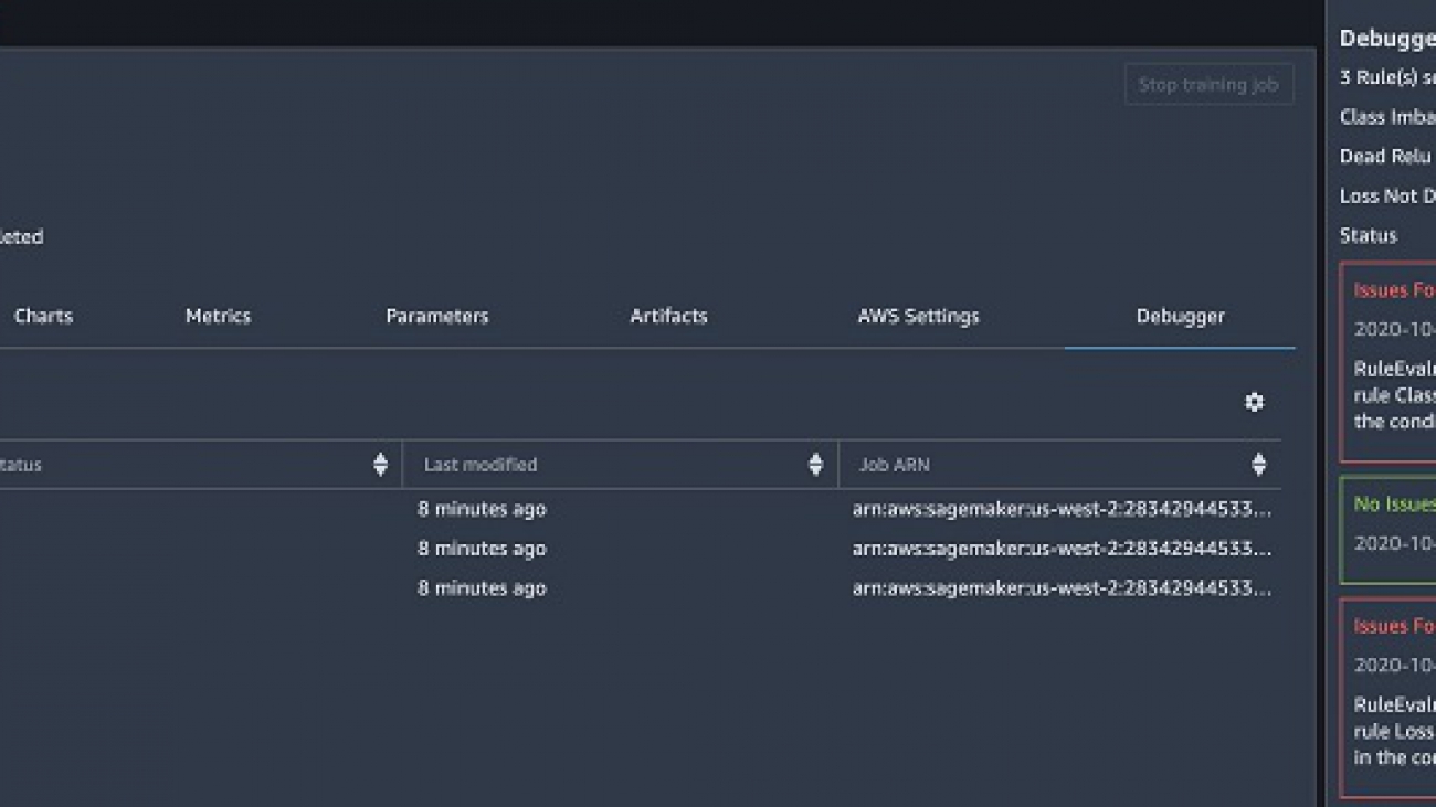
While the training is in progress, we can monitor the rule status in real time in Amazon SageMaker Studio. It turns out that the loss_not_decreasing and class_imbalance rules are triggered. The training runs for 10 epochs and reaches a final test accuracy of 96.3%.
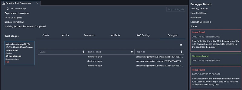
This seems good, but why were the rules triggered? Let’s dive into the data Debugger captured to find out the root causes.
Using SageMaker Debugger rules and data to uncover hidden problems
In this section, we investigate the data to find any hidden problems, create custom rules to fix the model, and rerun the training.
Inspecting loss_not_decreasing
We use Debugger to investigate what triggered the loss_not_decreasing rule. We use the smdebug library, which provides all the functionalities to read and access Debugger data. First we create a trial object that takes the path where the Debugger data is stored as input. This can either be a local or Amazon S3 path. With just a few lines of code, we can retrieve and visualize the loss values as training is still in progress. With trial.steps(), we retrieve the number of recorded steps: a step is one forward and backward pass. We can also specify a mode to retrieve data from the training (modes.TRAIN) or validation phase (modes.EVAL). Debugger’s default sampling interval is 500, so we get loss values for step 0, 500, 1,000, and so on.
To access the loss values, we pass the name of the loss into the trial.tensor() function. The cross entropy loss function we picked measures the performance of a multi-classification model. It takes two inputs: the model outputs and ground truth labels. We can access its outputs via trial.tensor('CrossEntropyLoss_output_0').values():
trial.tensor('CrossEntropyLoss_output_0').values(mode=modes.TRAIN)

{0: array(3.9195325, dtype=float32),
 500: array(0.8488243, dtype=float32),
 1000: array(0.54870504, dtype=float32),
 1500: array(0.25874993, dtype=float32),
 2000: array(0.20406848, dtype=float32),
 2500: array(0.29052508, dtype=float32),
 3000: array(0.18074727, dtype=float32),
 3500: array(0.1956144, dtype=float32),
 4000: array(0.2597512, dtype=float32)}
This code returns a dictionary in which the keys are the step numbers and the values are the loss values. We can now easily visualize the loss values as training is still in progress. See the following code:
import matplotlib.pyplot as plt
from smdebug.trials import create_trial

"path = pytorch_estimator.latest_job_debugger_artifacts_path()
create_trial(path)"

plt.ylabel('Train Loss')
plt.xlabel('Steps')
plt.plot(trial.steps(mode=modes.TRAIN),
         list(trial.tensor('CrossEntropyLoss_output_0').values(mode=modes.TRAIN).values()))
plt.show()
The blue curve in the following graph shows that the default training configuration ran the training for too long. Instead of training for 4,000 steps, early_stopping should have been applied after 1,000 steps. We can use Debugger to enable auto-termination, which stops the training when a rule triggers. For our use case, doing so reduces compute time by more than half (orange curve).
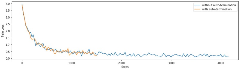
Debugger can auto-terminate training jobs. Metrics are sent to Amazon CloudWatch, so you can set up a CloudWatch alarm and AWS Lambda function that stops a training job if a rule triggers.
For more information about how the auto-termination feature helped one customer reduce compute costs by 70%, see Autodesk optimizes visual similarity search model in Fusion 360 with Amazon SageMaker Debugger.
Inspecting class_imbalance
Real-world datasets are often imbalanced and noisy. If the model training doesn’t account for these factors, it produces a model that has low or no predictive power for the classes with few samples. You can address this in different ways, such as during data-loading, when more samples can be drawn from the under-represented classes, or you can adjust the loss function to assign a higher penalty to incorrect predictions using class weights.
To investigate the class imbalance issue, we retrieve the inputs of the loss function (previously we retrieved the outputs) The loss function takes the model predictions and the ground truth labels as inputs. We use the latter (CrossEntropyLoss_input_1) to count the number of samples the model has seen during training:
from collections import Counter
labels = []
for step in trial.steps(mode=modes.TRAIN):
labels.extend(trial.tensor("CrossEntropyLoss_input_1").value(step, mode=modes.TRAIN))
label_counts = Counter(labels)
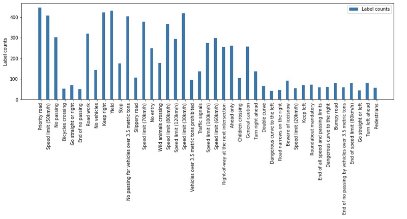
plt.bar(np.arange(0,43), label_counts.values()
The following visualization shows a high imbalance and several classes with fewer than a hundred samples.
To fix the class imbalance issue, we change the default configuration of the dataloaders to take the class weights into account and draw more samples from classes with fewer samples. Therefore, we define WeightedRandomSampler:
sampler = torch.utils.data.sampler.WeightedRandomSampler(weights, len(weights))

train_dataloader = torch.utils.data.DataLoader(dataset,
                                                batch_size=64,
                                                sampler=sampler)
During training, the dataloader now draws more samples from classes with lower counts. Class imbalance may lead to the problem where the model performs well on classes with a lot of samples but poorly on classes with fewer counts. Because we trained the model without WeightedRandomSampler, let’s see which classes had particularly low accuracy by looking at the confusion matrix.
Visualizing the confusion matrix in real time
To evaluate the performance of our model, we retrieve labels and predictions and create the confusion matrix:
from sklearn.metrics import confusion_matrix
import seaborn as sns

predictions = []
labels = []
for step in trial.steps(mode=modes.EVAL):
    predictions.extend(np.argmax(trial.tensor("CrossEntropyLoss_input_0").value(step, mode=modes.EVAL), axis=1))
    labels.extend(trial.tensor("CrossEntropyLoss_input_1").value(step, mode=modes.EVAL))

cm = confusion_matrix(labels,predictions)
sns.heatmap(cm, ax=ax, cbar=True)
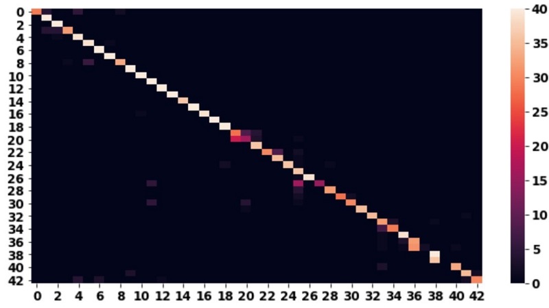
Each row in the matrix corresponds to the actual class, and the column indicates the predicted classes. For example, the first row shows class 0 and how often it was predicted as class 0, class 1, class 2, and so on. Ideally, we want high counts on the diagonal, because these are correctly predicted classes. Elements not on the diagonal are incorrect predictions. The confusion matrix helps us determine if particular classes in our dataset get confused more often with each other. This can happen, for instance, because samples from two different classes may be very similar. Debugger also provides a confusion built-in rule that computes the confusion matrix while the training is in progress and triggers if the ratio of data on-diagonal values and off-diagonal values exceeds a pre-defined threshold.
The following image shows that in most cases our model is predicting the correct classes, but there are a few outliers. You can use Debugger to look more closely into those outliers.
Inspecting incorrect model predictions
To find out what is causing those outliers in the confusion matrix, we investigate the examples upon which the model made false predictions. To do this analysis, we take both inputs into the loss function into account: CrossEntropyLoss_input_0 presents the model predictions, and CrossEntropyLoss_input_1 are the labels. We also retrieve the model inputs ResNet_input_0, which presents the input images. We perform the analysis on data recorded during the validation phase, so we specify mode=modes.EVAL.
We iterate over the predictions and model inputs saved by Debugger and select those where the label and prediction do not match. Then we plot the predictions and corresponding images:
for step in trial.steps(mode=modes.EVAL):

    predictions = np.argmax(trial.tensor('CrossEntropyLoss_input_0').value(step, mode=modes.EVAL),axis=1)
    labels = trial.tensor('CrossEntropyLoss_input_1').value(step, mode=modes.EVAL)
    images = trial.tensor('ResNet_input_0').value(step, mode=modes.EVAL)

    for prediction, label, image in zip(predictions, labels, images):
        if prediction != label:
            print(f"Predicted: '{signnames[p]}' Groundtruth: '{signnames[l]}' ")
            plt.imshow(i)
The following images show the result of the code segment. The analysis reveals that the model is often confused by traffic signs that involve a direction. Clearly this is a severe model bug despite the model achieving a decent test accuracy of 96.3%.
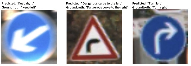
The root cause of this is the data augmentation pipeline, which performs a random horizontal flip on the training data. This data augmentation step is typically used when ResNet models are trained from scratch, but it causes a problem in our use case where the dataset contains similar classes where images just differ in their direction.
Running training with a custom rule
With Debugger, we can easily write a custom rule that checks how often the model was confused about directions. For example, we take the image “Dangerous curve to left” (class 19) and count how often it was mistaken as “Dangerous curve to right” (class 20) or vice versa. We just need to implement the function invoke_at_step that Debugger calls every time data for a new step is available. Like before, we access the inputs into the loss function: check if image class 19 or 20 is present, and count how often it was mistaken for the other. If this happens more than 10 times, the rule triggers. See the following code:
from smdebug.rules.rule import Rule

class MyCustomRule(Rule):
    def __init__(self, base_trial):
        super().__init__(base_trial)
        self.counter = 0

    def invoke_at_step(self, step):


        predictions = np.argmax(trial.tensor('CrossEntropyLoss_input_0').value(step),axis=1)
        labels = trial.tensor('CrossEntropyLoss_input_1').value(step)

        for prediction, label in zip(predictions, labels):

            if prediction == 19 and label == 20 or prediction == 20 and label == 19:
                self.counter += 1
                if self.counter > 10:
                    self.logger.info(f'Found {self.counter} cases where class 19 was mistaken as class 20 and vice versa')
                    return True

        return False
We can easily test and run the custom rule locally by creating the trial object and invoking the rule on the data:
from smdebug.rules import invoke_rule
from smdebug.exceptions import *

rule = MyCustomRule(trial)
try:
    invoke_rule(rule, raise_eval_cond=True)
except RuleEvaluationConditionMet as e:
    print(e)
Running the code cell in the notebook gives the following output:
[2020-10-18 18:51:24.588 28f0f34b9e29:12513 INFO rule_invoker.py:15] Started execution of rule MyCustomRule at step 0
[2020-10-18 18:53:11.846 28f0f34b9e29:12513 INFO <ipython-input-69-cae132ce9a97>:19] Found 11 cases where class 19 was mistaken as class 20 and vice versa
Evaluation of the rule MyCustomRule at step 1812 resulted in the condition being met
The rule triggered at step 1812. After the rule has been tested locally, we can run it as part of our Amazon SageMaker training job. First we need to save the rule in a separate file and then define the following configuration where we indicate on which instance type the rule should run:
from sagemaker.debugger import Rule, CollectionConfig

custom_rule = Rule.custom(
    name='MyCustomRule',
    image_uri='759209512951.dkr.ecr.us-west-2.amazonaws.com/sagemaker-debugger-rule-evaluator:latest',
    instance_type='ml.t3.medium',
    source='my_custom_rule.py',
    volume_size_in_gb=10,
    rule_to_invoke='MyCustomRule',
)
After we define the configuration, we add the custom_rule to the list of rules in the estimator object.
Fixing the model and rerunning training
Now that Debugger has helped us identify some critical issues in our model, we apply the fixes and rerun the training. As mentioned before, weighted re-sampling allows us to fix the class imbalance problem. We also change the data augmentation pipeline and remove the horizontal flip. We reduce the number of epochs from 10 to 3, because we have seen that the loss doesn’t decrease after roughly 1,000 iterations.
With Debugger, we can now compare data from different training jobs and see if the issues persist or not. We just need to create a new trial object, read data from both trials, and compare their tensors:
trial1 = create_trial("s3://bucket/training-job/debug-output")
trial2 = create_trial("s3://bucket/improved-training-job/debug-output")
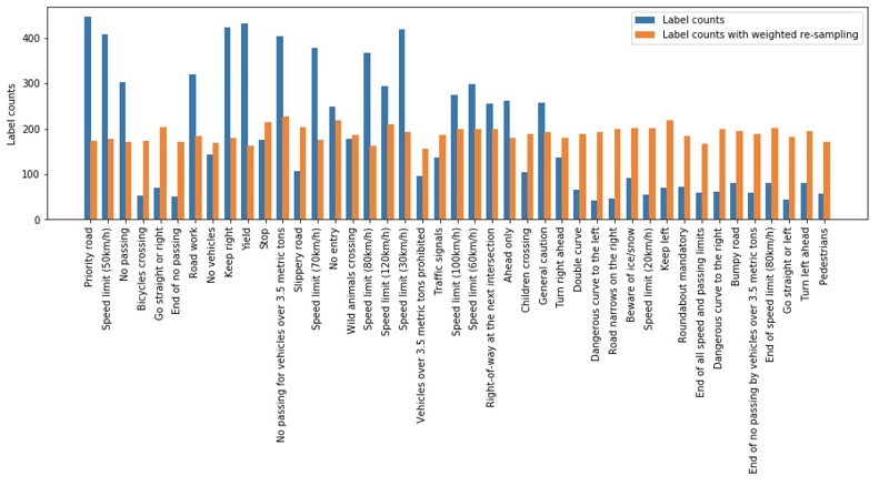
The following visualization shows the label counts for the original training job and the one where we applied weighted re-sampling (orange). We see that there is no longer a class imbalance issue and the model sees roughly the same amount of instances per class.
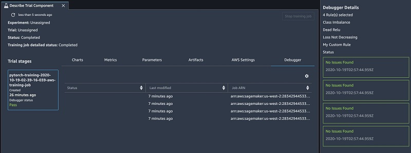
We run the training with the same built-in rules as before and add our own custom rule. We monitor the status of the rules and can now see that none of them trigger.
Summary
In this post, we have shown an end-to-end example of how to use Amazon SageMaker Debugger to automatically find, inspect, and fix issues in a deep neural network training.
As the state-of-the-art models grow in size and complexity, finding issues early in the prototyping phase is critical to save time and costs. Model bugs may not always be obvious and as we have shown in this post, a suboptimal model may still achieve an overall good accuracy.
In our use case, we not only found critical bugs, but also reduced training time by a factor of two and improved model performance.
There is no extra cost for running Debugger built-in rules, and you benefit by having them enabled because you may discover non-obvious model issues. If you want to learn more about Debugger, check out the following:
References
[1] Johannes Stallkamp, Marc Schlipsing, Jan Salmen, Christian Igel,
The German traffic sign recognition benchmark: A multi-class classification competition, The 2011 International Joint Conference on Neural Networks, 2011
About the Authors
 Nathalie Rauschmayr is an Applied Scientist at AWS, where she helps customers develop deep learning applications.
 Lu Huang is a Senior Product Manager on the AWS Deep Engine team, managing Sagemaker Debugger.
 Satadal Bhattacharjee is Principal Product Manager at AWS AI. He leads the machine learning engine PM team on projects such as SageMaker and optimizes machine learning frameworks such as TensorFlow, PyTorch, and MXNet.
Read More

 Taha A. Kass-Hout, MD, MS, is director of machine learning and chief medical officer at Amazon Web Services (AWS). Taha received his medical training at Beth Israel Deaconess Medical Center, Harvard Medical School, and during his time there, was part of the BOAT clinical trial. He holds a doctor of medicine and master’s of science (bioinformatics) from the University of Texas Health Science Center at Houston.
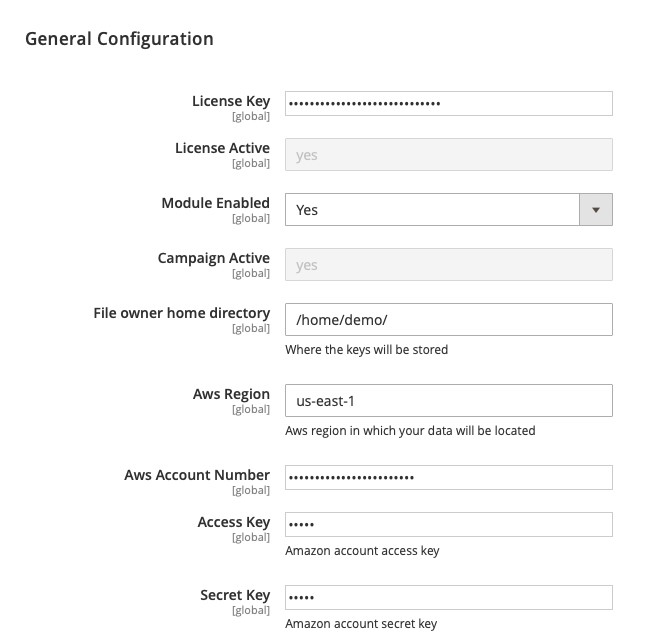
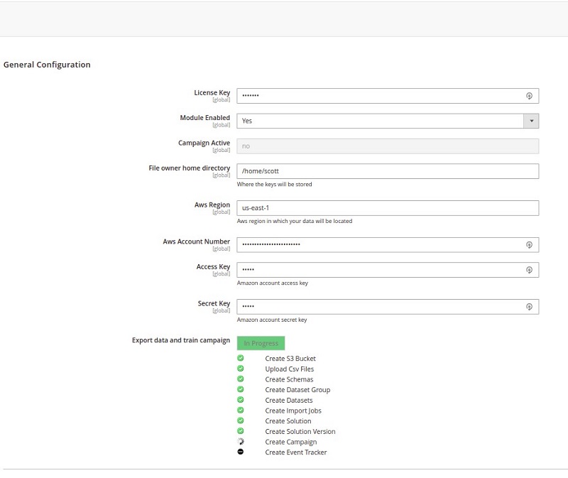
 If Enabled is set to No, Magento doesn’t use the extension.

 Rahul Suresh is an Engineering Manager with the AWS AI org, where he has been working on AI based products for making machine learning accessible for all developers. Prior to joining AWS, Rahul was a Senior Software Developer at Amazon Devices and helped launch highly successful smart home products. Rahul is passionate about building machine learning systems at scale and is always looking for getting these advanced technologies in the hands of customers. In addition to his professional career, Rahul is an avid reader and a history buff.
 Liang Li is an AI Researcher at AWS, where she works on AI based products to bring new cutting-edge ideas about Deep Learning to teach developers. Prior to joining AWS, Liang graduated from the University of Tennessee Knoxville with a Ph. D in EE, and she has been focusing on ML projects since graduation. In her spare time, she enjoys cooking and hiking.
 Suri Yaddanapudi is an AI Researcher and ML Engineer at AWS. He works on researching and implementing modern machine learning algorithms across different domains and teaching them to customers in a fun way. Prior to joining AWS, Suri graduated with his Ph.D. degree from University of Cincinnati and his thesis was focused on implementing AI techniques to Drug Repurposing. In his spare time, he enjoys reading, watching anime and playing futsal.


 Kashif Imran is a Principal Solutions Architect at Amazon Web Services. He works with some of the largest AWS customers who are taking advantage of AI/ML to solve complex business problems. He provides technical guidance and design advice to implement computer vision applications at scale. His expertise spans application architecture, serverless, containers, NoSQL and machine learning.
 Peter M. O’Donnell is an AWS Principal Solutions Architect, specializing in security, risk, and compliance with the Strategic Accounts team. Formerly dedicated to a major US commercial bank customer, Peter now supports some of AWS’s largest and most complex strategic customers in security and security-related topics, including data protection, cryptography, incident response, and CISO engagement.

 Dr. Yazdan Shirvany is all 12 AWS-certified Senior Solution Architect with deep experience in AI/ML, IOT and big data technologies including NLP, Knowledge Graph, applications reengineering, and optimizing software to leverage the cloud. Dr. Shirvany has 20+ scientific publications, and several issued patents in AI/ML field. Dr. Shirvany holds a M.S and Ph.D. in Computer Science from Chalmers University of Technology.
 Dipto Chakravarty is a leader in Amazon’s Alexa engineering group and heads up the Personal Mobility team in HQ2 utilizing AI, ML and IoT to solve local search analytics challenges. He has 12 patents issued to date and has authored two best-selling books on computer architecture and operating systems published by McGraw-Hill and Wiley. Dipto holds a B.S and M.S in Computer Science and Electrical Engineering from U. of Maryland, an EMBA from Wharton School, U. Penn, and a GMP from Harvard Business School.
 Mohit Mehta is a leader in the AWS Professional Services Organization with expertise in AI/ML and Big Data technologies. Mohit holds a M.S in Computer Science, all 12 AWS certifications, MBA from College of William and Mary and GMP from Michigan Ross School of Business.


 Guang Yang is a data scientist at the Amazon ML Solutions Lab where he works with customers across various verticals and applies creative problem solving to generate value for customers with state-of-the-art ML/AI solutions.