There have been breakthroughs in understanding COVID-19, such as how soon an exposed person will develop symptoms and how many people on average will contract the disease after contact with an exposed individual. The wider research community is actively working on accurately predicting the percent population who are exposed, recovered, or have built immunity. Researchers currently build epidemiology models and simulators using available data from agencies and institutions, as well as historical data from similar diseases such as influenza, SARS, and MERS. It’s an uphill task for any model to accurately capture all the complexities of the real world. Challenges in building these models include learning parameters that influence variations in disease spread across multiple countries or populations, being able to combine various intervention strategies (such as school closures and stay-at-home orders), and running what-if scenarios by incorporating trends from diseases similar to COVID-19. COVID-19 remains a relatively unknown disease with no historic data to predict trends.
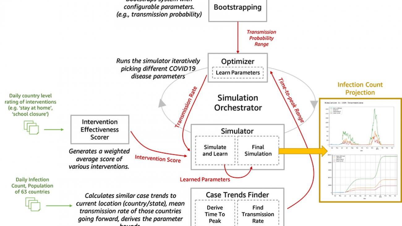
We are now open-sourcing a toolset for researchers and data scientists to better model and understand the progression of COVID-19 in a given community over time. This toolset is comprised of a disease progression simulator and several machine learning (ML) models to test the impact of various interventions. First, the ML models help bootstrap the system by estimating the disease progression and comparing the outcomes to historical data. Next, you can run the simulator with learned parameters to play out what-if scenarios for various interventions. In the following diagram, we illustrate the interactions among the extensible building blocks in the toolset.

In this post, we describe in detail how our disease simulation works, how simulation parameters are learned using supervised learning, and predict the incidence of disease given an intervention score.
Historical trends for infectious diseases
We provide several notebooks in our open-source toolset to run what-if scenarios at the state level in the US, India, and countries in Europe. In these notebooks, we use various data sources that frequently publish the number of new cases. For example, for the US, we use the Delphi Epidata API from Carnegie Mellon University (CMU) to access various datasets, including but not limited to the Johns Hopkins Center for Systems Science and Engineering (JHU-CSSE), survey trends from Google search and Facebook, and historical data for H1N1 in 2009–2010.
We can use our notebook, covid19_data_exploration.ipynb, to overlay historical data from previous pandemics with COVID-19. For example, the following graphs compare COVID-19 to seasonal flu and the H1N1 pandemic in California, Texas, and Illinois.
The first graph shows the 7-day average of the number of incidences in California during seasonal flu, H1N1, and COVID-19.

Although COVID-19 cases peaked in summer for most states in the US, there are exceptions. In Illinois, the most cases occurred early in the year, similar to the H1N1 peak in spring.

On the other hand, in other states such as Texas, we observe a potential peak aligning with the H1N1 peak in fall.

The trends differ greatly across states and countries. Therefore, we provide notebooks that enable you to run what-if scenarios by learning from existing data and projecting into the future using anticipated peaks.
Results from running what-if scenarios
The notebook covid19_simulator.ipynb has a comprehensive list of regions and countries across the world to run what-if scenarios. In this section, we discuss various what-if scenarios for France, Italy, the US, and Maharashtra, India. First, we use ML to predict the disease trends, including peaks and waves based on parameters specified by the user (for example, we use 3 months of COVID-19 case data to bootstrap and follow the H1N1 trend or create a second or third wave after 6 months from the first wave). Next, we play out intervention scenarios such as mild intervention or strict intervention and discuss the results.
France
For France, we considered the what-if scenario of having a stricter intervention and a second wave in 6 months but with a higher peak than the first wave, as expected in H1N1-like trends. The following graphs compare the daily number of cases and cumulative number of cases. Our projection in this scenario (orange line) closely matches with the actual curve (blue line).

Italy
For Italy, we consider the scenario of having a mild intervention policy versus a stricter intervention policy and a second wave in 6 months with a higher peak, as expected in H1N1-like trends. The first set of graphs shows the number of daily cases and total cases with a mild intervention policy.

The following graphs compare daily and total case numbers with a stricter intervention policy.

During the first wave, the milder intervention projection initially matches better, and stricter interventions result in a decline. Therefore, in this what-if scenario, we can see how our model captures varying interventions. However, although the trend with the second wave matches our predictions, using the assumption of a second wave in 6 months doesn’t align with the new trend. Therefore, the best projection for Italy’s what-if scenario should shift the second wave to where we usually expect H1N1 would have been—specifically, in fall.
US
For our US scenario, we considered having another wave in 3 months while keeping a stricter level of interventions. Overall, the US aligns better with stricter intervention scores based on the invention scoring mechanism provided by the Oxford Coronavirus Government Response Tracker, which we use for all the examples in this post and notebook. In this what-if scenario, we start observing a trend for another wave that aligns with H1N1-like trends in fall.

Maharashtra, India
Our Maharashtra, India, scenario considers having another wave in 6 months while keeping the same level of intervention policies. The graph on the left shows the actual (blue) and estimated (orange) number of cases. The graph the right is the cumulative number of cases. In this scenario, we can see the impact of experiencing a second wave is similar to the first one.

Disease simulator
We model the disease progression for each individual in a population using a finite state machine, and then report out the aggregate state of the population. We assign a probability distribution to the disease parameters for each individual, parametrized by a mean, standard deviation, and lower and upper limits. For example, you can set parameters such as individuals will develop symptoms within 2–5 days after exposure, with the majority of the population developing symptoms in 2–3 days. Similarly, you can set parameters for the recovery period, such as within 14–21 days after exposure. The stochasticity allows for variation in the population at the individual level to mimic real-world scenarios.
Our finite state machine is similar to the simulation model in COVID-19 Projections Using Machine Learning, with additional states for infection transmission by asymptomatic individuals, as shown in the following diagram. The default state machine is extensible in the sense that you can add any disease progression state to the model as long as the state transitions are well-defined from and to the new state. For example, you can add the state for having tested positive.

Our disease simulation can also capture population dynamics. The transition from one state to the next for an individual is influenced by the states of the others in the population. For example, a person transitions from a Susceptible to Exposed state based on factors such as whether the person is vulnerable due to pre-exiting health issues or interventions such as social distancing. Theoretically, our simulation model iterates each individual’s state within an automata network [4]. The state transition probabilities are driven by two types of factors:
- Individual, disease-specific factors – The probability densities assigned to the individual on how soon the symptoms will appear dictates transitioning from an Exposed state to Onset of systems
- Population, transmission-specific factors – The probability to transition from Susceptible to Exposed is higher for an individual with a larger social network or exposure to infected individuals
Learning simulation parameters
The simulation has different types of parameters. Some of these parameters are known or discovered by researchers and scientists, such as the number of days prior to the onset of symptoms. Other parameters such as transmission rate, which varies greatly among populations and rapidly over time, can be learned from actual data published by agencies. The following are three core simulation parameters learned by ML methods:
- Transmission rate – Transmission rate can be derived either directly from the recent case counts of the target location or as an expected value from the transmission rates of the countries matching the transmission rate pattern of the target location. As most of the regions (country / state / county) have now surpassed the peak of the 1st wave or already entered the 2nd wave, the transmission rate can be measured more reliably from respective country’s daily confirmed-cases data itself.
- Time (weeks) to reach the peak of the first wave of infection – This parameter can be learnt from the countries with matching transmission rate patterns. For those regions that are now beyond the peak of the 1st wave, this parameter can be captured by a sliding window analysis of the daily confirmed cases curve. In absence of sufficient matching countries, you can use a configurable range, such as 1–5 weeks.
- Transmission control – This parameter is learnt from a configurable range by reducing the simulation error for a validation timeframe with known case counts. 100% interventions can not prevent 100% transmission. Interventions tend to control only a fraction of the overall transmission scope. This parameter is intended to represent that fraction and can vary a lot across regions. It is learnt by fitting the wave-1 data against values from a range (e.g. 0.1 to 1) through iterative trial simulations.
Learning intervention scores
We score intervention effectiveness in the following three ways:
- Fitting score stringency index – Fits the daily intervention scores in a regression model with the OXCGRT-provided stringency index (
score_stringency_idx) as the dependent variable. Subsequently, it extracts the intervention effectiveness scores as the ensemble-based regression model’s feature importance. - Fitting confirmed case counts – Fits the daily intervention scores in a regression model with the changes in confirmed case counts (moving average) as the dependent variable. Feature importance scores indicate intervention effectiveness.
- Observing case count variations – Measures the changes in total case count by turning off the interventions one by one. Scores the interventions in proportion to the respective changes resulting from it being turned off.
Finally, these three scores can be combined using a configurable weighted average. Although these approaches would be affected by the co-occurrences and correlations among the interventions, as a whole, it can represent approximate relative effectiveness scores of the interventions.
Limitations of our toolset
Our toolset has the following limitations:
- Our disease model expects multiple waves of infections following Gaussian distribution, a pattern quite evident in past influenza pandemics [2].
- Our disease model doesn’t include death rates; however, it’s relatively straightforward to extend the finite state machine.
- Country-level intervention scores, to some extent, could be applicable at lower levels, like states, and thus have been used accordingly. However, a more accurate approach would be to gather and use the intervention scores at respective regional levels.
- The population size needs to be large enough due to underlying probabilistic components, such as 1,000 or more individuals.
- Although we assumed that on average one person can infect three people, based on a recent study published in Oxford Academic [cite], we anticipate this number to vary across populations. Therefore, it’s a configurable parameter in our base. Several studies indicate that individuals who don’t exhibit symptoms are the largest transmitters.
- Our model is designed to simulate the first 2 waves of the infection in our code repository and additional waves can be added as required.
Toolset architecture deep dive
In this section, we dive deep into the five main components of the toolset architecture.
- Bootstrapping – This block exposes the configurable parameters. The configurable parameters can be adjusted between 0.1 to 1.0. Similarly, wave1_weeks was initially 2 weeks; now its range is 1–5 weeks.
- Infection Wave(s) Analysis: We do a sliding window analysis of the smoothened daily confirmed cases data to detect the starting point and the peak of the 1st and 2nd. This information is subsequently used to infer the parameters of the underlying probability distributions that work at the core of the simulator.
- Intervention effectiveness scorer – We use supervised learning to estimate an intervention effectiveness score for a population using the research data from OXCGRT [1] or similar sources. Then we create a weighted average score.
- Optimizer – The optimization model iteratively varies the parameters to be learned and reduces the error in predicting the incidence rate based on the historical data.
- Predictions – After the simulation parameters are learned for a specific country or population, we can use the intervention effectiveness scores (the what-if scenario of a given disease progression pattern over time, such as the second peak in June) to run our simulation to predict the relative impact of an intervention in future.
Toolset inputs and outputs
The inputs are as follows:
- Daily infection counts from over 60 countries
- Daily country-level rating of over 10 interventions, such as stay-at-home orders or school closures
- A disease incidence pattern with peaks and their timing and duration
- Simulation duration
Our output is the incidence rate over the course of the simulation.
Summary
Our open-source code simulates COVID-19 case projections at various regional granularity levels. The output is the projection of the total confirmed cases over a specific timeline for a target state or a country, for a given degree of intervention.
Our solution first tries to understand the approximate time to peak and expected case rates of the daily COVID-19 cases for the target entity (state/country) by analysis of the disease incidence patterns. Next, it selects the best (optimal) parameters using optimization techniques on a simulation model. Finally, it generates the projections of daily and cumulative confirmed cases, starting from the beginning of the outbreak uptil a specified length of time in the future.
To get started, we have provided a few sample simulations at state and country levels in the covid19_simulator.ipynb notebook in https://github.com/aws-samples/covid19-simulation, which you can run on Amazon SageMaker or a local environment.
References
[1] Oxford Coronavirus Government Response Tracker https://www.bsg.ox.ac.uk/research/research-projects/coronavirus-government-response-tracker [2] Mummert A, Weiss H, Long LP, Amigó JM, Wan XF (2013) A Perspective on Multiple Waves of Influenza Pandemics. PLOS ONE 8(4): e60343. https://doi.org/10.1371/journal.pone.0060343 [3] Viceconte, Giulio, and Nicola Petrosillo. “COVID-19 R0: Magic number or conundrum?.” Infectious disease reports vol. 12,1 8516. 24 Feb. 2020, doi:10.4081/idr.2020.8516 https://www.ncbi.nlm.nih.gov/pmc/articles/PMC7073717/ [4] https://nyuscholars.nyu.edu/en/publications/automata-networks-and-artificial-intelligence)FAQs
Q. What is incidence rate vs. prevalence rate?
Incidence refers to the occurrence of new cases of disease or injury in a population over a specified period of time. Incidence rate is a measure of incidence that incorporates time directly into the denominator. Prevalence differs from incidence, in that prevalence includes all cases, both new and pre-existing, in the population at the specified time, whereas incidence is limited to new cases only.
Q. How are the interventions effectiveness scored?
Interventions effectiveness can be scored in the following three ways:
- Fitting score stringency index – Fits the daily intervention scores in a regression model with the OXCGRT-provided stringency index (
score_stringency_idx) as the dependent variable. Subsequently, it extracts the intervention effectiveness scores as the ensemble-based regression model’s feature importance. - Fitting confirmed case counts – Fits the daily intervention scores in a regression model with the changes in confirmed case counts (moving average) as the dependent variable. Feature importance scores indicate intervention effectiveness.
- Observing case count variations – Measures the changes in total case count by turning off the interventions one by one. Scores the interventions in proportion to the respective changes resulting from it being turned off.
Finally, these three scores can be combined using a configurable weighted average. Although these approaches would be affected by the co-occurrences and correlations among the interventions, as a whole, it can represent an approximate relative effectiveness scores of the interventions.
Q. How are we computing expected transmission rate and time to peak?
Given the latest case rate and transmission rate growth patterns of a region, the solution first identifies the countries that have exhibited similar patterns in the past and eventually plateaued. From these reference countries, it determines the time-to-peak and mean/median daily growth rates until the peak. When a considerable number (default 5) of countries found with matching patterns, then the expected transmission rate, and time-to-peak are computed as weighted averages using pattern and population similarity levels.
Q. What parameters are learned?
The solution always learns the transmission probability for the location in context (country or state) by fitting the simulation model outcome against the confirmed case counts. Optionally, it can also learn the optimal time (in weeks) to reach the peak of the infection spread. Prior to optimization, the time to reach the peak is approximated from the data of other countries having similar transmission patterns.
Q. Can the simulation work starting at any point of the disease progression timeline?
No. One of the key parameters in the solution is the recent transmission rate change (growth). If the simulation starts at a very early stage of disease progression, the transmission rate might be too low to come up with realistic future projections. Similarly, if the simulation starts at the plateau or declining phase, the transmission rate change might be negative and therefore generate incorrect projections. This solution works best on the moderate-to-high-growth phase of the disease progression.
About the Authors
 Tomal Deb is a Data Scientist in the Amazon Machine Learning Solutions Lab. He has worked on a wide range of data science problems involving NLP, Recommender Systems, Forecasting , Numerical Optimization, etc.
 Sahika Genc is a Principal Applied Scientist in the AWS AI team. Her current research focus is deep reinforcement learning (RL) for smart automation and robotics. Previously, she was a senior research scientist in the Artificial Intelligence and Learning Laboratory at the General Electric (GE) Global Research Center, where she led science teams on healthcare analytics for patient monitoring.
 Sunil Mallya is a Principal Deep Learning Scientist in the AWS AI team. He leads engineering for Amazon Comprehend and enjoys solving problems in the area of NLP. In addition, Sunil also enjoys working on Reinforcement Learning and Autonomous Cars.
 Atanu Roy is a Principal Deep Learning Architect in the Amazon ML Solutions Lab and leads the team for India. He spends most of his spare time and money on his solo travels.
 Vinay Hanumaiah is a Deep Learning Architect at Amazon ML Solutions Lab, where he helps customers build AI and ML solutions to accelerate their business challenges. Prior to this, he contributed to the launch of AWS DeepLens and Amazon Personalize. In his spare time, he enjoys time with his family and is an avid rock climber.
 Nate Slater leads the US West and APAC/Japan/China business for the Amazon Machine Learning Solutions Lab.
 Taha A. Kass-Hout, MD, MS, is General Manager, Machine Learning & Chief Medical Officer at Amazon Web Services (AWS).


 Shanthan Kesharaju is a Senior Architect who helps our customers with AI/ML strategy and architecture. Shanthan has an MBA in Marketing from Duke University and an MS in Management Information Systems from Oklahoma State University.
 Blake DeLee is a Rochester, NY-based conversational AI consultant with AWS Professional Services. He has spent five years in the field of conversational AI and voice, and has experience bringing innovative solutions to dozens of Fortune 500 businesses. Blake draws on a wide-ranging career in different fields to build exceptional chatbot and voice solutions.


 Ben Snively is an AWS Public Sector Specialist Solutions Architect. He works with government, non-profit, and education customers on big data/analytical and AI/ML projects, helping them build solutions using AWS.
 Sam Palani is an AI/ML Specialist Solutions Architect at AWS. He works with public sector customers to help them architect and implement machine learning solutions at scale. When not helping customers, he enjoys long hikes, unwinding with a good book, listening to his classical vinyl collection and hacking projects with Raspberry Pi.