Posts in category: Amazon AWS

KT Corporation is one of the largest telecommunications providers in South Korea, offering a wide range of services including fixed-line telephone, mobile communication, and internet, and AI services. KT’s AI Food Tag is an AI-based dietary management solution that identifies the type and nutritional content of food in photos using a computer vision model. This vision model developed by KT relies on a model pre-trained with a large amount of unlabeled image data to analyze the nutritional content and calorie information of various foods. The AI Food Tag can help patients with chronic diseases such as diabetes manage their diets. KT used AWS and Amazon SageMaker to train this AI Food Tag model 29 times faster than before and optimize it for production deployment with a model distillation technique. In this post, we describe KT’s model development journey and success using SageMaker.

Introducing the KT project and defining the problem

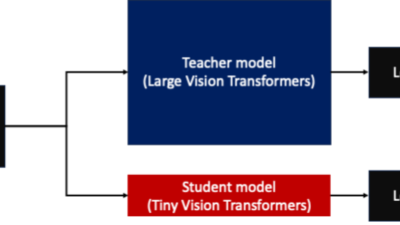
The AI Food Tag model pre-trained by KT is based on the vision transformers (ViT) architecture and has more model parameters than their previous vision model to improve accuracy. To shrink the model size for production, KT is using a knowledge distillation (KD) technique to reduce the number of model parameters without significant impact to accuracy. With knowledge distillation, the pre-trained model is called a teacher model, and a lightweight output model is trained as a student model, as illustrated in the following figure. The lightweight student model has fewer model parameters than the teacher, which reduces memory requirements and allows for deployment on smaller, less expensive instances. The student maintains acceptable accuracy even though it’s smaller by learning from the outputs of the teacher model.

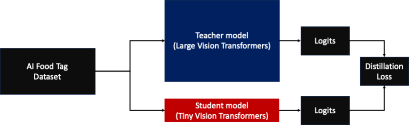
The teacher model remains unchanged during KD, but the student model is trained using the output logits of the teacher model as labels to calculate loss. With this KD paradigm, both the teacher and the student need to be on a single GPU memory for training. KT initially used two GPUs (A100 80 GB) in their internal, on-premises environment to train the student model, but the process took about 40 days to cover 300 epochs. To accelerate training and generate a student model in less time, KT partnered with AWS. Together, the teams significantly reduced model training time. This post describes how the team used Amazon SageMaker Training, the SageMaker Data Parallelism Library, Amazon SageMaker Debugger, and Amazon SageMaker Profiler to successfully develop a lightweight AI Food Tag model.

Building a distributed training environment with SageMaker

SageMaker Training is a managed machine learning (ML) training environment on AWS that provides a suite of features and tools to simplify the training experience and can be useful in distributed computing, as illustrated in the following diagram.

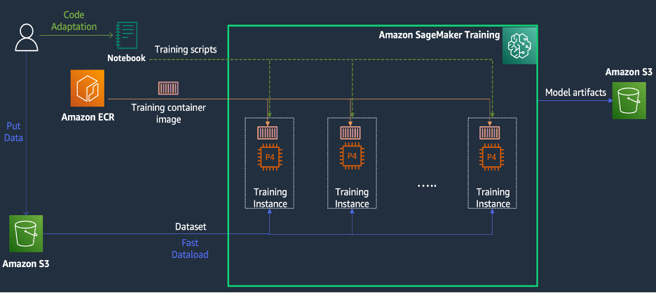
SageMaker customers can also access built-in Docker images with various pre-installed deep learning frameworks and the necessary Linux, NCCL, and Python packages for model training. Data scientists or ML engineers who want to run model training can do so without the burden of configuring training infrastructure or managing Docker and the compatibility of different libraries.

During a 1-day workshop, we were able to set up a distributed training configuration based on SageMaker within KT’s AWS account, accelerate KT’s training scripts using the SageMaker Distributed Data Parallel (DDP) library, and even test a training job using two ml.p4d.24xlarge instances. In this section, we describe KT’s experience working with the AWS team and using SageMaker to develop their model.

In the proof of concept, we wanted to speed up a training job by using the SageMaker DDP library, which is optimized for AWS infrastructure during distributed training. To change from PyTorch DDP to SageMaker DDP, you simply need to declare the torch_smddp package and change the backend to smddp, as shown in the following code:

import smdistributed.dataparallel.torch.torch_smddp

dist.init_process_group(backend='smddp',

rank=args.rank,

world_size=args.world_size)

To learn more about the SageMaker DDP library, refer to SageMaker’s Data Parallelism Library.

Analyzing the causes of slow training speed with the SageMaker Debugger and Profiler

The first step in optimizing and accelerating a training workload involves understanding and diagnosing where bottlenecks occur. For KT’s training job, we measured the training time per iteration of the data loader, forward pass, and backward pass:

Looking at the time in the standard output for each iteration, we saw that the backward pass’s run time fluctuated significantly from iteration to iteration. This variation is unusual and can impact total training time. To find the cause of this inconsistent training speed, we first tried to identify resource bottlenecks by utilizing the System Monitor (SageMaker Debugger UI), which allows you to debug training jobs on SageMaker Training and view the status of resources such as the managed training platform’s CPU, GPU, network, and I/O within a set number of seconds.

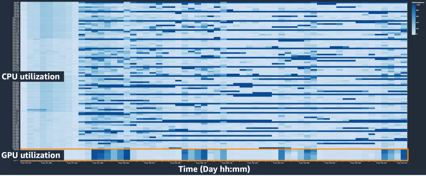
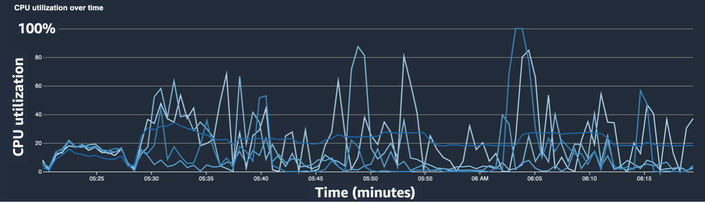
The SageMaker Debugger UI provides detailed and essential data that can help identifying and diagnose bottlenecks in a training job. Specifically, the CPU utilization line chart and CPU/GPU utilization heat map per instance tables caught our eye.

In the CPU utilization line chart, we noticed that some CPUs were being used 100%.

In the heat map (where darker colors indicate higher utilization), we noted that a few CPU cores had high utilization throughout the training, whereas GPU utilization wasn’t consistently high over time.

From here, we began to suspect that one of the reasons for the slow training speed was a CPU bottleneck. We reviewed the training script code to see if anything was causing the CPU bottleneck. The most suspicious part was the large value of num_workers in the data loader, so we changed this value to 0 or 1 to reduce CPU utilization. We then ran the training job again and checked the results.

The following screenshots show the CPU utilization line chart, GPU utilization, and heat map after mitigating the CPU bottleneck.

By simply changing num_workers, we saw a significant decrease in CPU utilization and an overall increase in GPU utilization. This was an important change that improved training speed significantly. Still, we wanted to see where we could optimize GPU utilization. For this, we used SageMaker Profiler.

SageMaker Profiler helps identify optimization clues by providing visibility into utilization by operations, including tracking GPU and CPU utilization metrics and kernel consumption of GPU/CPU within training scripts. It helps users understand which operations are consuming resources. First, to use SageMaker Profiler, you need to add ProfilerConfig to the function that invokes the training job using the SageMaker SDK, as shown in the following code:

from sagemaker import ProfilerConfig, Profiler

from sagemaker.debugger import (ProfilerRule, rule_configs)

rules=[ProfilerRule.sagemaker(rule_configs.ProfilerReport())]

profiler_config = ProfilerConfig(profile_params = Profiler(cpu_profiling_duration=3600))

from sagemaker.pytorch import PyTorch

region_name = 'us-west-2'

image_uri=f'763104351884.dkr.ecr.{region_name}.amazonaws.com/pytorch-training:2.0.0-gpu-py310-cu118-ubuntu20.04-sagemaker'

estimator = PyTorch(

entry_point='train.py',

source_dir='src',

role=role,

image_uri=image_uri,

instance_count=4,

instance_type='ml.p4d.24xlarge',

distribution={'smdistributed': {'dataparallel': {'enabled': True}}},

profiler_config=profiler_config,

hyperparameters=hyperparameters,

sagemaker_session=sagemaker_session,

)

In the SageMaker Python SDK, you have the flexibility to add the annotate functions for SageMaker Profiler to select code or steps in the training script that needs profiling. The following is an example of the code that you should declare for SageMaker Profiler in the training scripts:

import smppy

SMProf = smppy.SMProfiler.instance()

config = smppy.Config()

config.profiler = {

"EnableCuda": "1",

}

SMProf.configure(config)

SMProf.start_profiling()

…

with smppy.annotate("Forward"):

student_out = student_model(inp)

with smppy.annotate("Backward"):

loss.backward()

…

SMProf.stop_profiling()

After adding the preceding code, if you run a training job using the training scripts, you can get information about the operations consumed by the GPU kernel (as shown in the following figure) after the training runs for a period of time. In the case of KT’s training scripts, we ran it for one epoch and got the following results.

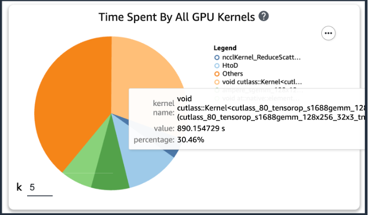
When we checked the top five operation consumption times of the GPU kernel among the results of SageMaker Profiler, we found that for the KT training script, the most time is consumed by the matrix product operation, which is a general matrix multiplication (GEMM) operation on GPUs. With this important insight from the SageMaker Profiler, we began investigating ways to accelerate these operations and improve GPU utilization.

Speeding up training time

We reviewed various ways to reduce computation time of matrix multiplication and applied two PyTorch functions.

Shard optimizer states with ZeroRedundancyOptimizer

If you look at the Zero Redundancy Optimizer (ZeRO), the DeepSpeed/ZeRO technique enables the training of a large model efficiently with better training speed by eliminating the redundancies in memory used by the model. ZeroRedundancyOptimizer in PyTorch uses the technique of sharding the optimizer state to reduce memory usage per a process in Distributed Data Parallel (DDP). DDP uses synchronized gradients in the backward pass so that all optimizer replicas iterate over the same parameters and gradient values, but instead of having all the model parameters, each optimizer state is maintained by sharding only for different DDP processes to reduce memory usage.

To use it, you can leave your existing Optimizer in optimizer_class and declare a ZeroRedundancyOptimizer with the rest of the model parameters and the learning rate as parameters.

student_optimizer = ZeroRedundancyOptimizer(

student_model.parameters(),

optimizer_class=torch.optim.AdamW,

lr=initial_lr

)

Automatic mixed precision

Automatic mixed precision (AMP) uses the torch.float32 data type for some operations and torch.bfloat16 or torch.float16 for others, for the convenience of fast computation and reduced memory usage. In particular, because deep learning models are typically more sensitive to exponent bits than fraction bits in their computations, torch.bfloat16 is equivalent to the exponent bits of torch.float32, allowing them to learn quickly with minimal loss. torch.bfloat16 only runs on instances with A100 NVIDIA architecture (Ampere) or higher, such as ml.p4d.24xlarge, ml.p4de.24xlarge, and ml.p5.48xlarge.

To apply AMP, you can declare torch.cuda.amp.autocast in the training scripts as shown in the code above and declare dtype as torch.bfloat16.

with torch.cuda.amp.autocast(dtype="torch.bfloat16"):

teacher = teacher_model(input_data)

student = student_model(input_data)

loss = loss(teacher, student, target)

loss.requires_grad_(True)

loss.backward()

student_optimizer.step()

student_optimizer.zero_grad(set_to_none=True)

Results in SageMaker Profiler

After applying the two functions to the training scripts and running a train job for one epoch again, we checked the top five operations consumption times for the GPU kernel in SageMaker Profiler. The following figure shows our results.

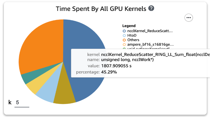
We can see that the GEMM operation, which was at the top of the list before applying the two Torch functions, has disappeared from the top five operations, replaced by the ReduceScatter operation, which typically occurs in distributed training.

Training speed results of the KT distilled model

We increased the training batch size by 128 more to account for the memory savings from applying the two Torch functions, resulting in a final batch size of 1152 instead of 1024. The training of the final student model was able to run 210 epochs per 1 day; the training time and speedup between KT’s internal training environment and SageMaker are summarized in the following table.

The scalability of AWS allowed us to complete the training job 29 times faster than before using 32 GPUs instead of 2 on premises. As a result, using more GPUs on SageMaker would have significantly reduced training time with no difference in overall training costs.

Conclusion

Park Sang-min (Vision AI Serving Technology Team Leader) from the AI2XL Lab in KT’s Convergence Technology Center commented on the collaboration with AWS to develop the AI Food Tag model:

“Recently, as there are more transformer-based models in the vision field, the model parameters and required GPU memory are increasing. We are using lightweight technology to solve this issue, and it takes a lot of time, about a month to learn once. Through this PoC with AWS, we were able to identify the resource bottlenecks with help of SageMaker Profiler and Debugger, resolve them, and then use SageMaker’s data parallelism library to complete the training in about one day with optimized model code on four ml.p4d.24xlarge instances.”

SageMaker helped save Sang-min’s team weeks of time in model training and development.

Based on this collaboration on the vision model, AWS and the SageMaker team will continue to collaborate with KT on various AI/ML research projects to improve model development and service productivity through applying SageMaker capabilities.

To learn more about related features in SageMaker, check out the following:

• Train machine learning models
• SageMaker’s Data Parallelism Library
• Use Amazon SageMaker Debugger to debug and improve model performance
• Use Amazon SageMaker Profiler to profile activities on AWS compute resources

About the authors

Youngjoon Choi, AI/ML Expert SA, has experienced enterprise IT in various industries such as manufacturing, high-tech, and finance as a developer, architect, and data scientist. He conducted research on machine learning and deep learning, specifically on topics like hyperparameter optimization and domain adaptation, presenting algorithms and papers. At AWS, he specializes in AI/ML across industries, providing technical validation using AWS services for distributed training/large scale models and building MLOps. He proposes and reviews architectures, aiming to contribute to the expansion of the AI/ML ecosystem.

Jung Hoon Kim is an account SA of AWS Korea. Based on experiences in applications architecture design, development and systems modeling in various industries such as hi-tech, manufacturing, finance and public sector, he is working on AWS Cloud journey and workloads optimization on AWS for enterprise customers.

Rock Sakong is a researcher at KT R&D. He has conducted research and development for the vision AI in various fields and mainly conducted facial attributes (gender/glasses, hats, etc.)/face recognition technology related to the face. Currently, he is working on lightweight technology for the vision models.

Manoj Ravi is a Senior Product Manager for Amazon SageMaker. He is passionate about building next-gen AI products and works on software and tools to make large-scale machine learning easier for customers. He holds an MBA from Haas School of Business and a Masters in Information Systems Management from Carnegie Mellon University. In his spare time, Manoj enjoys playing tennis and pursuing landscape photography.

Robert Van Dusen is a Senior Product Manager with Amazon SageMaker. He leads frameworks, compilers, and optimization techniques for deep learning training.

Read More

Amazon Interactive Video Service (Amazon IVS) is a managed live streaming solution that is designed to provide a quick and straightforward setup to let you build interactive video experiences and handles interactive video content from ingestion to delivery.

With the increased usage of live streaming, the need for effective content moderation becomes even more crucial. User-generated content (UGC) presents complex challenges for safety. Many companies rely on human moderators to monitor video streams, which is time-consuming, error-prone, and doesn’t scale with business growth speed. An automated moderation solution supporting a human in the loop (HITL) is increasingly needed.

Amazon Rekognition Content Moderation, a capability of Amazon Rekognition, automates and streamlines image and video moderation workflows without requiring machine learning (ML) experience. In this post, we explain the common practice of live stream visual moderation with a solution that uses the Amazon Rekognition Image API to moderate live streams. You can deploy this solution to your AWS account using the AWS Cloud Development Kit (AWS CDK) package available in our GitHub repo.

Moderate live stream visual content

The most common approach for UGC live stream visual moderation involves sampling images from the stream and utilizing image moderation to receive near-real-time results. Live stream platforms can use flexible rules to moderate visual content. For instance, platforms with younger audiences might have strict rules about adult content and certain products, whereas others might focus on hate symbols. These platforms establish different rules to match their policies effectively. Combining human and automatic review, a hybrid process is a common design approach. Certain streams will be stopped automatically, but human moderators will also assess whether a stream violates platform policies and should be deactivated.

The following diagram illustrates the conceptual workflow of a near-real-time moderation system, designed with loose coupling to the live stream system.

The workflow contains the following steps:

1. The live stream service (or the client app) samples image frames from video streams based on a specific interval.
2. A rules engine evaluates moderation guidelines, determining the frequency of stream sampling and the applicable moderation categories, all within predefined policies. This process involves the utilization of both ML and non-ML algorithms.
3. The rules engine alerts human moderators upon detecting violations in the video streams.
4. Human moderators assess the result and deactivate the live stream.

Moderating UGC live streams is distinct from classic video moderation in media. It caters to diverse regulations. How frequently images are sampled from video frames for moderation is typically determined by the platform’s Trust & Safety policy and the service-level agreement (SLA). For instance, if a live stream platform aims to stop channels within 3 minutes for policy violations, a practical approach is to sample every 1–2 minutes, allowing time for human moderators to verify and take action. Some platforms require flexible moderation frequency control. For instance, highly reputable streamers may need less moderation, whereas new ones require closer attention. This also enables cost-optimization by reducing sampling frequency.

Cost is an important consideration in any live stream moderation solution. As UGC live stream platforms rapidly expand, moderating concurrent streams at a high frequency can raise cost concerns. The solution presented in this post is designed to optimize cost by allowing you to define moderation rules to customize sample frequency, ignore similar image frames, and other techniques.

Recording Amazon IVS stream content to Amazon S3

Amazon IVS offers native solutions for recording stream content to an Amazon Simple Storage Service (Amazon S3) bucket and generating thumbnails—image frames from a video stream. It generates thumbnails every 60 seconds by default and provides users the option to customize the image quality and frequency. Using the AWS Management Console, you can create a recording configuration and link it to an Amazon IVS channel. When a recording configuration is associated with a channel, the channel’s live streams are automatically recorded to the specified S3 bucket.

There are no Amazon IVS charges for using the auto-record to Amazon S3 feature or for writing to Amazon S3. There are charges for Amazon S3 storage, Amazon S3 API calls that Amazon IVS makes on behalf of the customer, and serving the stored video to viewers. For details about Amazon IVS costs, refer to Costs (Low-Latency Streaming).

Amazon Rekognition Moderation APIs

In this solution, we use the Amazon Rekognition DetectModerationLabel API to moderate Amazon IVS thumbnails in near-real time. Amazon Rekognition Content Moderation provides pre-trained APIs to analyze a wide range of inappropriate or offensive content, such as violence, nudity, hate symbols, and more. For a comprehensive list of Amazon Rekognition Content Moderation taxonomies, refer to Moderating content.

The following code snippet demonstrates how to call the Amazon Rekognition DetectModerationLabel API to moderate images within an AWS Lambda function using the Python Boto3 library:

import boto3

# Initialize the Amazon Rekognition client object
rekognition = boto3.client('rekognition')

# Call the Rekognition Image moderation API
response = rekognition.detect_moderation_labels(
 Image={'S3Object': {'Bucket': data_bucket,'Name': s3_key}}
)

The following is an example response from the Amazon Rekognition Image Moderation API:

{
    "ModerationLabels": [
        {
            "Confidence": 99.9290542602539,
            "Name": "Female Swimwear Or Underwear",
            "ParentName": "Suggestive"
        },
        ...
    ],
    "ModerationModelVersion": "6.1"
}

For additional examples of the Amazon Rekognition Image Moderation API, refer to our Content Moderation Image Lab.

Solution overview

This solution integrates with Amazon IVS by reading thumbnail images from an S3 bucket and sending images to the Amazon Rekognition Image Moderation API. It provides choices for stopping the stream automatically and human-in-the-loop review. You can configure rules for the system to automatically halt streams based on conditions. It also includes a light human review portal, empowering moderators to monitor streams, manage violation alerts, and stop streams when necessary.

In this section, we briefly introduce the system architecture. For more detailed information, refer to the GitHub repo.

The following screen recording displays the moderator UI, enabling them to monitor active streams with moderation warnings, and take actions such as stopping the stream or dismissing warnings.

Users can customize moderation rules, controlling video stream sample frequency per channel, configuring Amazon Rekognition moderation categories with confidence thresholds, and enabling similarity checks, which ensures performance and cost-optimization by avoiding processing redundant images.

The following screen recording displays the UI for managing a global configuration.

The solution uses a microservices architecture, which consists of two key components loosely coupled with Amazon IVS.

Rules engine

The rules engine forms the backbone of the live stream moderation system. It is a live processing service that enables near-real-time moderation. It uses Amazon Rekognition to moderate images, validates results against customizable rules, employs image hashing algorithms to recognize and exclude similar images, and can halt streams automatically or alert the human review subsystem upon rule violations. The service integrates with Amazon IVS through Amazon S3-based image reading and facilitates API invocation via Amazon API Gateway.

The following architecture diagram illustrates the near-real-time moderation workflow.

There are two methods to trigger the rules engine processing workflow:

• S3 file trigger – When a new image is added to the S3 bucket, the workflow starts. This is the recommended way for Amazon IVS integration.
• REST API call – You can make a RESTful API call to API Gateway with the image bytes in the request body. The API stores the image in an S3 bucket, triggering near-real-time processing. This approach is fitting for images captured by the client side of the live stream app and transmitted over the internet.

The image processing workflow, managed by AWS Step Functions, involves several steps:

1. Check the sample frequency rule. Processing halts if the previous sample time is too recent.
2. If enabled in the config, perform a similarity check using image hash algorithms. The process skips the image if it’s similar to the previous one received for the same channel.
3. Use the Amazon Rekognition Image Moderation API to assess the image against configured rules, applying a confidence threshold and ignoring unnecessary categories.
4. If the moderation result violates any rules, send notifications to an Amazon Simple Notification Service (Amazon SNS) topic, alerting downstream systems with moderation warnings.
5. If the auto stop moderation rule is violated, the Amazon IVS stream will be stopped automatically.

The design manages rules through a Step Functions state machine, providing a drag-and-drop GUI for flexible workflow definition. You can extend the rules engine by incorporating additional Step Functions workflows.

Monitoring and management dashboard

The monitoring and management dashboard is a web application with a UI that lets human moderators monitor Amazon IVS live streams. It provides near-real-time moderation alerts, allowing moderators to stop streams or dismiss warnings. The web portal also empowers administrators to manage moderation rules for the rules engine. It supports two types of configurations:

• Channel rules – You can define rules for specific channels.
• Global rules – These rules apply to all or a subset of Amazon IVS channels that lack specific configurations. You can define a regular expression to apply the global rule to Amazon IVS channel names matching a pattern. For example: .* applies to all channels. /^test-/ applies to channels with names starting with test-.

The system is a serverless web app, featuring a static React front end hosted on Amazon S3 with Amazon CloudFront for caching. Authentication is handled by Amazon Cognito. Data is served through API Gateway and Lambda, with state storage in Amazon DynamoDB. The following diagram illustrates this architecture.

The monitoring dashboard is a lightweight demo app that provides essential features for moderators. To enhance functionality, you can extend the implementation to support multiple moderators with a management system and reduce latency by implementing a push mechanism using WebSockets.

Moderation latency

The solution is designed for near-real-time moderation, with latency measured across two separate subsystems:

• Rules engine workflow – The rules engine workflow, from receiving images to sending notifications via Amazon SNS, averages within 2 seconds. This service promptly handles images through a Step Functions state machine. The Amazon Rekognition Image Moderation API processes under 500 milliseconds for average file sizes below 1 MB. (These findings are based on tests conducted with the sample app, meeting near-real-time requirements.) In Amazon IVS, you have the option to select different thumbnail resolutions to adjust the image size.
• Monitoring web portal – The monitoring web portal subscribes to the rules engine’s SNS topic. It records warnings in a DynamoDB table, while the website UI fetches the latest warnings every 10 seconds. This design showcases a lightweight demonstration of the moderator’s view. To further reduce latency, consider implementing a WebSocket to instantly push warnings to the UI upon their arrival via Amazon SNS.

Extend the solution

This post focuses on live stream visual content moderation. However, the solution is intentionally flexible, capable of accommodating complex business rules and extensible to support other media types, including moderating chat messages and audio in live streams. You can enhance the rules engine by introducing new Step Functions state machine workflows with upstream dispatching logic. We’ll delve deeper into live stream text and audio moderation using AWS AI services in upcoming posts.

Summary

In this post, we provided an overview of a sample solution that showcases how to moderate Amazon IVS live stream videos using Amazon Rekognition. You can experience the sample app by following the instructions in the GitHub repo and deploying it to your AWS account using the included AWS CDK package.

Learn more about content moderation on AWS. Take the first step towards streamlining your content moderation operations with AWS.

About the Authors

Lana Zhang is a Senior Solutions Architect at AWS WWSO AI Services team, specializing in AI and ML for Content Moderation, Computer Vision, Natural Language Processing and Generative AI. With her expertise, she is dedicated to promoting AWS AI/ML solutions and assisting customers in transforming their business solutions across diverse industries, including social media, gaming, e-commerce, media, advertising & marketing.

Tony Vu is a Senior Partner Engineer at Twitch. He specializes in assessing partner technology for integration with Amazon Interactive Video Service (IVS), aiming to develop and deliver comprehensive joint solutions to our IVS customers.

Read More

Generative AI models have the potential to revolutionize enterprise operations, but businesses must carefully consider how to harness their power while overcoming challenges such as safeguarding data and ensuring the quality of AI-generated content.

The Retrieval-Augmented Generation (RAG) framework augments prompts with external data from multiple sources, such as document repositories, databases, or APIs, to make foundation models effective for domain-specific tasks. This post presents the capabilities of the RAG model and highlights the transformative potential of MongoDB Atlas with its Vector Search feature.

MongoDB Atlas is an integrated suite of data services that accelerate and simplify the development of data-driven applications. Its vector data store seamlessly integrates with operational data storage, eliminating the need for a separate database. This integration enables powerful semantic search capabilities through Vector Search, a fast way to build semantic search and AI-powered applications.

Amazon SageMaker enables enterprises to build, train, and deploy machine learning (ML) models. Amazon SageMaker JumpStart provides pre-trained models and data to help you get started with ML. You can access, customize, and deploy pre-trained models and data through the SageMaker JumpStart landing page in Amazon SageMaker Studio with just a few clicks.

Amazon Lex is a conversational interface that helps businesses create chatbots and voice bots that engage in natural, lifelike interactions. By integrating Amazon Lex with generative AI, businesses can create a holistic ecosystem where user input seamlessly transitions into coherent and contextually relevant responses.

Solution overview

The following diagram illustrates the solution architecture.

In the following sections, we walk through the steps to implement this solution and its components.

Set up a MongoDB cluster

To create a free tier MongoDB Atlas cluster, follow the instructions in Create a Cluster. Set up the database access and network access.

Deploy the SageMaker embedding model

You can choose the embedding model (ALL MiniLM L6 v2) on the SageMaker JumpStart Models, notebooks, solutions page.

Choose Deploy to deploy the model.

Verify the model is successfully deployed and verify the endpoint is created.

Vector embedding

Vector embedding is a process of converting a text or image into a vector representation. With the following code, we can generate vector embeddings with SageMaker JumpStart and update the collection with the created vector for every document:

payload = {"text_inputs": [document[field_name_to_be_vectorized]]}
query_response = query_endpoint_with_json_payload(json.dumps(payload).encode('utf-8'))
embeddings = parse_response_multiple_texts(query_response)

# update the document
update = {'$set': {vector_field_name :  embeddings[0]}}
collection.update_one(query, update)

The code above shows how to update a single object in a collection.  To update all objects follow the instructions.

MongoDB vector data store

MongoDB Atlas Vector Search is a new feature that allows you to store and search vector data in MongoDB. Vector data is a type of data that represents a point in a high-dimensional space. This type of data is often used in ML and artificial intelligence applications. MongoDB Atlas Vector Search uses a technique called k-nearest neighbors (k-NN) to search for similar vectors. k-NN works by finding the k most similar vectors to a given vector. The most similar vectors are the ones that are closest to the given vector in terms of the Euclidean distance.

Storing vector data next to operational data can improve performance by reducing the need to move data between different storage systems. This is especially beneficial for applications that require real-time access to vector data.

Create a Vector Search index

The next step is to create a MongoDB Vector Search index on the vector field you created in the previous step. MongoDB uses the knnVector type to index vector embeddings. The vector field should be represented as an array of numbers (BSON int32, int64, or double data types only).

Refer to Review knnVector Type Limitations for more information about the limitations of the knnVector type.

The following code is a sample index definition:

{
  "mappings": {
    "dynamic": true,
    "fields": {
      "egVector": {
        "dimensions": 384,
        "similarity": "euclidean",
        "type": "knnVector"
      }
    }
  }
}

Note that the dimension must match you embeddings model dimension.

Query the vector data store

You can query the vector data store using the Vector Search aggregation pipeline. It uses the Vector Search index and performs a semantic search on the vector data store.

The following code is a sample search definition:

{
  $search: {
    "index": "<index name>", // optional, defaults to "default"
    "knnBeta": {
      "vector": [<array-of-numbers>],
      "path": "<field-to-search>",
      "filter": {<filter-specification>},
      "k": <number>,
      "score": {<options>}
    }
  }
}

Deploy the SageMaker large language model

SageMaker JumpStart foundation models are pre-trained large language models (LLMs) that are used to solve a variety of natural language processing (NLP) tasks, such as text summarization, question answering, and natural language inference. They are available in a variety of sizes and configurations. In this solution, we use the Hugging Face FLAN-T5-XL model.

Search for the FLAN-T5-XL model in SageMaker JumpStart.

Choose Deploy to set up the FLAN-T5-XL model.

Verify the model is deployed successfully and the endpoint is active.

Create an Amazon Lex bot

To create an Amazon Lex bot, complete the following steps:

1. On the Amazon Lex console, choose Create bot.

1. For Bot name, enter a name.
2. For Runtime role, select Create a role with basic Amazon Lex permissions.
   
3. Specify your language settings, then choose Done.
   
4. Add a sample utterance in the NewIntent UI and choose Save intent.
   
5. Navigate to the FallbackIntent that was created for you by default and toggle Active in the Fulfillment section.
   
6. Choose Build and after the build is successful, choose Test.
   
7. Before testing, choose the gear icon.
   
8. Specify the AWS Lambda function that will interact with MongoDB Atlas and the LLM to provide responses.  To create the lambda function follow these steps.
   
9. You can now interact with the LLM.

Clean up

To clean up your resources, complete the following steps:

1. Delete the Amazon Lex bot.
2. Delete the Lambda function.
3. Delete the LLM SageMaker endpoint.
4. Delete the embeddings model SageMaker endpoint.
5. Delete the MongoDB Atlas cluster.

Conclusion

In the post, we showed how to create a simple bot that uses MongoDB Atlas semantic search and integrates with a model from SageMaker JumpStart. This bot allows you to quickly prototype user interaction with different LLMs in SageMaker Jumpstart while pairing them with the context originating in MongoDB Atlas.

As always, AWS welcomes feedback. Please leave your feedback and questions in the comments section.

About the authors

Igor Alekseev is a Senior Partner Solution Architect at AWS in Data and Analytics domain. In his role Igor is working with strategic partners helping them build complex, AWS-optimized architectures. Prior joining AWS, as a Data/Solution Architect he implemented many projects in Big Data domain, including several data lakes in Hadoop ecosystem. As a Data Engineer he was involved in applying AI/ML to fraud detection and office automation.

Babu Srinivasan is a Senior Partner Solutions Architect at MongoDB. In his current role, he is working with AWS to build the technical integrations and reference architectures for the AWS and MongoDB solutions. He has more than two decades of experience in Database and Cloud technologies . He is passionate about providing technical solutions to customers working with multiple Global System Integrators(GSIs) across multiple geographies.

Read More

From enhancing the conversational experience to agent assistance, there are plenty of ways that generative artificial intelligence (AI) and foundation models (FMs) can help deliver faster, better support. With the increasing availability and diversity of FMs, it’s difficult to experiment and keep up-to-date with the latest model versions. Amazon Bedrock is a fully managed service that offers a choice of high-performing FMs from leading AI companies such as AI21 Labs, Anthropic, Cohere, Meta, Stability AI, and Amazon. With Amazon Bedrock’s comprehensive capabilities, you can easily experiment with a variety of top FMs, customize them privately with your data using techniques such as fine-tuning and Retrieval Augmented Generation (RAG).

Agents for Amazon Bedrock

In July, AWS announced the preview of agents for Amazon Bedrock, a new capability for developers to create fully managed agents in a few clicks. Agents extend FMs to run complex business tasks—from booking travel and processing insurance claims to creating ad campaigns and managing inventory—all without writing any code. With fully managed agents, you don’t have to worry about provisioning or managing infrastructure.

In this post, we provide a step-by-step guide with building blocks to create a customer service bot. We use a text generation model (Anthropic Claude V2) and agents for Amazon Bedrock for this solution. We provide an AWS CloudFormation template to provision the resources needed for building this solution. Then we walk you through steps to create an agent for Amazon Bedrock.

ReAct Prompting

FMs determine how to solve user-requested tasks with a technique called ReAct. It’s a general paradigm that combines reasoning and acting with FMs. ReAct prompts FMs to generate verbal reasoning traces and actions for a task. This allows the system to perform dynamic reasoning to create, maintain, and adjust plans for acting while incorporating additional information into the reasoning. The structured prompts include a sequence of question-thought-action-observation examples.

• The question is the user-requested task or problem to solve.
• The thought is a reasoning step that helps demonstrate to the FM how to tackle the problem and identify an action to take.
• The action is an API that the model can invoke from an allowed set of APIs.
• The observation is the result of carrying out the action.

Components in agents for Amazon Bedrock

Behind the scenes, agents for Amazon Bedrock automate the prompt engineering and orchestration of user-requested tasks. They can securely augment the prompts with company-specific information to provide responses back to the user in natural language. The agent breaks the user-requested task into multiple steps and orchestrates subtasks with the help of FMs. Action groups are tasks that the agent can perform autonomously. Action groups are mapped to an AWS Lambda function and related API schema to perform API calls. The following diagram depicts the agent structure.

Solution overview

We use a shoe retailer use case to build the customer service bot. The bot helps customers purchase shoes by providing options in a humanlike conversation. Customers converse with the bot in natural language with multiple steps invoking external APIs to accomplish subtasks. The following diagram illustrates the sample process flow.

The following diagram depicts a high-level architecture of this solution.

1. You can create an agent with Amazon Bedrock-supported FMs such as Anthropic Claude V2.
2. Attach API schema, residing in an Amazon Simple Storage Service (Amazon S3) bucket, and a Lambda function containing the business logic to the agent. (Note: This is a one-time setup step.)
3. The agent uses customer requests to create a prompt using the ReAct framework. It, then, uses the API schema to invoke corresponding code in the Lambda function.
4. You can perform a variety of tasks, including sending email notifications, writing to databases, and triggering application APIs in the Lambda functions.

In this post, we use the Lambda function to retrieve customer details, list shoes matching customer-preferred activity, and finally, place orders. Our code is backed by an in-memory SQLite database. You can use similar constructs to write to a persistent data store.

Prerequisites

To implement the solution provided in this post, you should have an AWS account and access to Amazon Bedrock with agents enabled (currently in preview). Use AWS CloudFormation template to create the resource stack needed for the solution.

us-east-1

The CloudFormation template creates two IAM roles. Update these roles to apply least-privilege permissions as discussed in Security best practices. Click here to learn what IAM features are available to use with agents for Amazon Bedrock.

1. LambdaBasicExecutionRole with Amazon S3 full access and CloudWatch access for logging.
2. AmazonBedrockExecutionRoleForAgents with Amazon S3 full access and Lambda full access.

Important: Agents for Amazon Bedrock must have the role name prefixed by AmazonBedrockExecutionRoleForAgents_*

Bedrock Agents setup

In the next two sections, we will walk you through creating and testing an agent.

Create an agent for Amazon Bedrock

To create an agent, open the Amazon Bedrock console and choose Agents in the left navigation pane. Then select Create Agent.

This starts the agent creation workflow.

1. Provide agent details: Give the agent a name and description (optional). Select the service role created by the CloudFormation stack and select Next.

2. Select a foundation model: In the Select model screen, you select a model. Provide clear and precise instructions to the agent about what tasks to perform and how to interact with the users.

3. Add action groups: An action is a task the agent can perform by making API calls. A set of actions comprise an action group. You provide an API schema that defines all the APIs in the action group. You must provide an API schema in the OpenAPI schema JSON format. The Lambda function contains the business logic needed to perform API calls. You must associate a Lambda function to each action group.

Give the action group a name and a description for the action. Select the Lambda function, provide an API schema file and select Next.

4. In the final step, review the agent configuration and select Create Agent.

Test and deploy agents for Amazon Bedrock

1. Test the agent: After the agent is created, a dialog box shows the agent overview along with a working draft. The Amazon Bedrock console provides a UI to test your agent.

2. Deploy: After successful testing, you can deploy your agent. To deploy an agent in your application, you must create an alias. Amazon Bedrock then automatically creates a version for that alias.

The following actions occur with the preceding agent setup and the Lambda code provided with this post:

1. The agent creates a prompt from the developer-provided instructions (such as “You are an agent that helps customers purchase shoes.”), API schemas needed to complete the tasks, and data source details. The automatic prompt creation saves weeks of experimenting with prompts for different FMs.
2. The agent orchestrates the user-requested task, such as “I am looking for shoes,” by breaking it into smaller subtasks such as getting customer details, matching the customer-preferred activity with shoe activity, and placing shoe orders. The agent determines the right sequence of tasks and handles error scenarios along the way.

The following screenshot displays some example responses from the agent.

By selecting Show trace for each response, a dialog box shows the reasoning technique used by the agent and the final response generated by the FM.

Cleanup

To avoid incurring future charges, delete the resources. You can do this by deleting the stack from the CloudFormation console.

Feel free to download and test the code used in this post from the GitHub agents for Amazon Bedrock repository. You can also invoke the agents for Amazon Bedrock programmatically; an example Jupyter Notebook is provided in the repository.

Conclusion

Agents for Amazon Bedrock can help you increase productivity, improve your customer service experience, or automate DevOps tasks. In this post, we showed you how to set up agents for Amazon Bedrock to create a customer service bot.

We encourage you to learn more by reviewing additional features of Amazon Bedrock. You can use the example code provided in this post to create your implementation. Try our workshop to gain hands-on experience with Amazon Bedrock.

About the Authors

Amit Arora is an AI and ML Specialist Architect at Amazon Web Services, helping enterprise customers use cloud-based machine learning services to rapidly scale their innovations. He is also an adjunct lecturer in the MS data science and analytics program at Georgetown University in Washington D.C.

Manju Prasad is a Senior Solutions Architect within Strategic Accounts at Amazon Web Services. She focuses on providing technical guidance in a variety of domains, including AI/ML to a marquee M&E customer. Prior to joining AWS, she has worked for companies in the Financial Services sector and also a startup.

Archana Inapudi is a Senior Solutions Architect at AWS supporting Strategic Customers. She has over a decade of experience helping customers design and build data analytics, and database solutions. She is passionate about using technology to provide value to customers and achieve business outcomes.

Read More

This is a joint blog with AWS and Philips.

Philips is a health technology company focused on improving people’s lives through meaningful innovation. Since 2014, the company has been offering customers its Philips HealthSuite Platform, which orchestrates dozens of AWS services that healthcare and life sciences companies use to improve patient care. It partners with healthcare providers, startups, universities, and other companies to develop technology that helps doctors make more precise diagnoses and deliver more personalized treatment for millions of people worldwide.

One of the key drivers of Philips’ innovation strategy is artificial intelligence (AI), which enables the creation of smart and personalized products and services that can improve health outcomes, enhance customer experience, and optimize operational efficiency.

Amazon SageMaker provides purpose-built tools for machine learning operations (MLOps) to help automate and standardize processes across the ML lifecycle. With SageMaker MLOps tools, teams can easily train, test, troubleshoot, deploy, and govern ML models at scale to boost productivity of data scientists and ML engineers while maintaining model performance in production.

In this post, we describe how Philips partnered with AWS to develop AI ToolSuite—a scalable, secure, and compliant ML platform on SageMaker. This platform provides capabilities ranging from experimentation, data annotation, training, model deployments, and reusable templates. All these capabilities are built to help multiple lines of business innovate with speed and agility while governing at scale with central controls. We outline the key use cases that provided requirements for the first iteration of the platform, the core components, and the outcomes achieved. We conclude by identifying the ongoing efforts to enable the platform with generative AI workloads and rapidly onboard new users and teams to adopt the platform.

Customer context

Philips uses AI in various domains, such as imaging, diagnostics, therapy, personal health, and connected care. Some examples of AI-enabled solutions that Philips has developed over the past years are:

• Philips SmartSpeed – An AI-based imaging technology for MRI that uses a unique Compressed-SENSE based deep learning AI algorithm to take speed and image quality to the next level for a large variety of patients
• Philips eCareManager – A telehealth solution that uses AI to support the remote care and management of critically ill patients in intensive care units, by using advanced analytics and clinical algorithms to process the patient data from multiple sources, and providing actionable insights, alerts, and recommendations for the care team
• Philips Sonicare – A smart toothbrush that uses AI to analyze the brushing behavior and oral health of users, and provide real-time guidance and personalized recommendations, such as optimal brushing time, pressure, and coverage, to improve their dental hygiene and prevent cavities and gum diseases.

For many years, Philips has been pioneering the development of data-driven algorithms to fuel its innovative solutions across the healthcare continuum. In the diagnostic imaging domain, Philips developed a multitude of ML applications for medical image reconstruction and interpretation, workflow management, and treatment optimization. Also in patient monitoring, image guided therapy, ultrasound and personal health teams have been creating ML algorithms and applications. However, innovation was hampered due to using fragmented AI development environments across teams. These environments ranged from individual laptops and desktops to diverse on-premises computational clusters and cloud-based infrastructure. This heterogeneity initially enabled different teams to move fast in their early AI development efforts, but is now holding back opportunities to scale and improve efficiency of our AI development processes.

It was evident that a fundamental shift towards a unified and standardized environment was imperative to truly unleash the potential of data-driven endeavors at Philips.

Key AI/ML use cases and platform requirements

AI/ML-enabled propositions can transform healthcare by automating administrative tasks done by clinicians. For example:

• AI can analyze medical images to help radiologists diagnose diseases faster and more accurately
• AI can predict future medical events by analyzing patient data and improving proactive care
• AI can recommend personalized treatment tailored to patients’ needs
• AI can extract and structure information from clinical notes to make record-taking more efficient
• AI interfaces can provide patient support for queries, reminders, and symptom checkers

Overall, AI/ML promises reduced human error, time and cost savings, optimized patient experiences, and timely, personalized interventions.

One of the key requirements for the ML development and deployment platform was the ability of the platform to support the continuous iterative development and deployment process, as shown in the following figure.

The AI asset development starts in a lab environment, where the data is collected and curated, and then the models are trained and validated. When the model is ready and approved for use, it’s deployed into the real-world production systems. Once deployed, model performance is continuously monitored. The real-world performance and feedback are eventually used for further model improvements with full automation of the model training and deployment.

The more detailed AI ToolSuite requirements were driven by three example use cases:

• Develop a computer vision application aimed at object detection at the edge. The data science team expected an AI-based automated image annotation workflow to speed up a time-consuming labeling process.
• Enable a data science team to manage a family of classic ML models for benchmarking statistics across multiple medical units. The project required automation of model deployment, experiment tracking, model monitoring, and more control over the entire process end to end both for auditing and retraining in the future.
• Improve the quality and time to market for deep learning models in diagnostic medical imaging. The existing computing infrastructure didn’t allow for running many experiments in parallel, which delayed model development. Also, for regulatory purposes, it’s necessary to enable full reproducibility of model training for several years.

Non-functional requirements

Building a scalable and robust AI/ML platform requires careful consideration of non-functional requirements. These requirements go beyond the specific functionalities of the platform and focus on ensuring the following:

• Scalability – The AI ToolSuite platform must be able to scale Philips’s insights generation infrastructure more effectively so that the platform can handle a growing volume of data, users, and AI/ML workloads without sacrificing performance. It should be designed to scale horizontally and vertically to meet increasing demands seamlessly while providing central resource management.
• Performance – The platform must deliver high-performance computing capabilities to efficiently process complex AI/ML algorithms. SageMaker offers a wide range of instance types, including instances with powerful GPUs, which can significantly accelerate model training and inference tasks. It also should minimize latency and response times to provide real-time or near-real-time results.
• Reliability – The platform must provide a highly reliable and robust AI infrastructure that spans across multiple Availability Zones. This multi-AZ architecture should ensure uninterrupted AI operations by distributing resources and workloads across distinct data centers.
• Availability – The platform must be available 24/7, with minimal downtime for maintenance and upgrades. AI ToolSuite’s high availability should include load balancing, fault-tolerant architectures, and proactive monitoring.
• Security and Governance – The platform must employ robust security measures, encryption, access controls, dedicated roles, and authentication mechanisms with continuous monitoring for unusual activities and conducting security audits.
• Data Management – Efficient data management is crucial for AI/ML platforms. Regulations in the healthcare industry call for especially rigorous data governance. It should include features like data versioning, data lineage, data governance, and data quality assurance to ensure accurate and reliable results.
• Interoperability – The platform should be designed to integrate easily with Philips’s internal data repositories, allowing seamless data exchange and collaboration with third-party applications.
• Maintainability – The platform’s architecture and code base should be well organized, modular, and maintainable. This enables Philips ML engineers and developers to provide updates, bug fixes, and future enhancements without disrupting the entire system.
• Resource optimization – The platform should monitor utilization reports very closely to make sure computing resources are used efficiently and allocate resources dynamically based on demand. In addition, Philips should use AWS Billing and Cost Management tools to make sure teams receive notifications when utilization passes the allocated threshold amount.
• Monitoring and logging – The platform should use Amazon CloudWatch alerts for comprehensive monitoring and logging capabilities, which are necessary to track system performance, identify bottlenecks, and troubleshoot issues effectively.
• Compliance – The platform can also help improve regulatory compliance of AI-enabled propositions. Reproducibility and traceability must be enabled automatically by the end-to-end data processing pipelines, where many mandatory documentation artifacts, such as data lineage reports and model cards, can be prepared automatically.
• Testing and validation – Rigorous testing and validation procedures must be in place to ensure the accuracy and reliability of AI/ML models and prevent unintended biases.

Solution overview

AI ToolSuite is an end-to-end, scalable, quick start AI development environment offering native SageMaker and associated AI/ML services with Philips HealthSuite security and privacy guardrails and Philips ecosystem integrations. There are three personas with dedicated sets of access permissions:

• Data scientist – Prepare data, and develop and train models in a collaborative workspace
• ML engineer – Productionize ML applications with model deployment, monitoring, and maintenance
• Data science admin – Create a project per team request to provide dedicated isolated environments with use case-specific templates

The platform development spanned multiple release cycles in an iterative cycle of discover, design, build, test, and deploy. Due to the uniqueness of some applications, the extension of the platform required embedding existing custom components like data stores or proprietary tools for annotation.
The following figure illustrates the three-layer architecture of AI ToolSuite, including the base infrastructure as the first layer, common ML components as the second layer, and project-specific templates as the third layer.

Layer 1 contains the base infrastructure:

• A networking layer with parametrized access to the internet with high availability
• Self-service provisioning with infrastructure as code (IaC)
• An integrated development environment (IDE) using an Amazon SageMaker Studio domain
• Platform roles (data science admin, data scientist)
• Artifacts storage
• Logging and monitoring for observability

Layer 2 contains common ML components:

• Automated experiment tracking for every job and pipeline
• A model build pipeline to launch a new model build update
• A model training pipeline comprised of model training, evaluation, registration
• A model deploy pipeline to deploy the model for final testing and approval
• A model registry to easily manage model versions
• A project role created specifically for a given use case, to be assigned to SageMaker Studio users
• An image repository for storing processing, training, and inference container images built for the project
• A code repository to store code artifacts
• A project Amazon Simple Storage Service (Amazon S3) bucket to store all project data and artifacts

Layer 3 contains project-specific templates that can be created with custom components as required by new projects. For example:

• Template 1 – Includes a component for data querying and history tracking
• Template 2 – Includes a component for data annotations with a custom annotation workflow to use proprietary annotation tooling
• Template 3 – Includes components for custom container images to customize both their development environment and training routines, dedicated HPC file system, and access from a local IDE for users

The following diagram highlights the key AWS services spanning multiple AWS accounts for development, staging, and production.

In the following sections, we discuss the key capabilities of the platform enabled by AWS services, including SageMaker, AWS Service Catalog, CloudWatch, AWS Lambda, Amazon Elastic Container Registry (Amazon ECR), Amazon S3, AWS Identity and Access Management (IAM), and others.

Infrastructure as code

The platform uses IaC, which allows Philips to automate the provisioning and management of infrastructure resources. This approach will also help reproducibility, scalability, version control, consistency, security, and portability for development, testing, or production.

Access to AWS environments

SageMaker and associated AI/ML services are accessed with security guardrails for data preparation, model development, training, annotation, and deployment.

Isolation and collaboration

The platform ensures data isolation by storing and processing separately, reducing the risk of unauthorized access or data breaches.

The platform facilitates team collaboration, which is essential in AI projects that typically involve cross-functional teams, including data scientists, data science admins, and MLOps engineers.

Role-based access control

Role-based access control (RBAC) is essential in managing permissions and simplifying access management by defining roles and permissions in a structured manner. It makes it straightforward to manage permissions as teams and projects grow and access control for different personas involved in AWS AI/ML projects, such as the data science admin, data scientist, annotation admin, annotator, and MLOps engineer.

Access to data stores

The platform allows SageMaker access to data stores, which ensures that data can be efficiently utilized for model training and inference without the need to duplicate or move data across different storage locations, thereby optimizing resource utilization and reducing costs.

Annotation using Philips-specific annotation tools

AWS offers a suite of AI and ML services, such as SageMaker, Amazon SageMaker Ground Truth, and Amazon Cognito, which are fully integrated with Philips-specific in-house annotation tools. This integration enables developers to train and deploy ML models using the annotated data within the AWS environment.

ML templates

The AI ToolSuite platform offers templates in AWS for various ML workflows. These templates are preconfigured infrastructure setups tailored to specific ML use cases and are accessible through services like SageMaker project templates, AWS CloudFormation, and Service Catalog.

Integration with Philips GitHub

Integration with GitHub enhances efficiency by providing a centralized platform for version control, code reviews, and automated CI/CD (continuous integration and continuous deployment) pipelines, reducing manual tasks and boosting productivity.

Visual Studio Code integration

Integration with Visual Studio Code provides a unified environment for coding, debugging, and managing ML projects. This streamlines the entire ML workflow, reducing context switching and saving time. The integration also enhances collaboration among team members by enabling them to work on SageMaker projects together within a familiar development environment, utilizing version control systems, and sharing code and notebooks seamlessly.

Model and data lineage and traceability for reproducibility and compliance

The platform provides versioning, which helps keep track of changes to the data scientist’s training and inference data over time, making it easier to reproduce results and understand the evolution of the datasets.

The platform also enables SageMaker experiment tracking, which allows end-users to log and track all the metadata associated with their ML experiments, including hyperparameters, input data, code, and model artifacts. These capabilities are essential for demonstrating compliance with regulatory standards and ensuring transparency and accountability in AI/ML workflows.

AI/ML specification report generation for regulatory compliance

AWS maintains compliance certifications for various industry standards and regulations. AI/ML specification reports serve as essential compliance documentation, showcasing adherence to regulatory requirements. These reports document the versioning of datasets, models, and code. Version control is essential for maintaining data lineage, traceability, and reproducibility, all of which are critical for regulatory compliance and auditing.

Project-level budget management

Project-level budget management allows the organization to set limits on spending, helping to avoid unexpected costs and ensuring that the ML projects stay within budget. With budget management, the organization can allocate specific budgets to individual projects or teams, which helps teams identify resource inefficiencies or unexpected cost spikes early on. In addition to budget management, with the feature to automatically shut down idle notebooks, team members avoid paying for unused resources, also releasing valuable resources when they are not actively in use, making them available for other tasks or users.

Outcomes

AI ToolSuite was designed and implemented as an enterprise-wide platform for ML development and deployment for data scientists across Philips. Diverse requirements from all business units were collected and considered during the design and development. Early in the project, Philips identified champions from the business teams who provided feedback and helped evaluate the value of the platform.

The following outcomes were achieved:

• User adoption is one of the key leading indicators for Philips. Users from several business units were trained and onboarded to the platform, and that number is expected to grow in 2024.
• Another important metric is the efficiency for data science users. With AI ToolSuite, new ML development environments are deployed in less than an hour instead of several days.
• Data science teams can access a scalable, secure, cost-efficient, cloud-based compute infrastructure.
• Teams can run multiple model training experiments in parallel, which significantly reduced the average training time from weeks to 1–3 days.
• Because the environment deployment is fully automated, it requires virtually no involvement of the cloud infrastructure engineers, which reduced operational costs.
• The use of AI ToolSuite significantly enhanced the overall maturity of data and AI deliverables by promoting the use of good ML practices, standardized workflows, and end-to-end reproducibility, which is critical for regulatory compliance in the healthcare industry.

Looking forward with generative AI

As organizations race to adopt the next state-of-the-art in AI, it’s imperative to adopt new technology in the context of the organization’s security and governance policy. The architecture of AI ToolSuite provides an excellent blueprint for enabling access to generative AI capabilities in AWS for different teams at Philips. Teams can use foundation models made available with Amazon SageMaker JumpStart, which provides a vast number of open source models from Hugging Face and other providers. With the necessary guardrails already in place in terms of access control, project provisioning, and cost controls, it will be seamless for teams to start using the generative AI capabilities within SageMaker.

Additionally, access to Amazon Bedrock, a fully managed API-driven service for generative AI, can be provisioned for individual accounts based on project requirements, and the users can access Amazon Bedrock APIs either via the SageMaker notebook interface or through their preferred IDE.

There are additional considerations concerning the adoption of generative AI in a regulated setting, such as healthcare. Careful consideration needs to be given to the value created by generative AI applications against the associated risks and costs. There is also a need to create a risk and legal framework that governs the organization’s use of generative AI technologies. Elements such as data security, bias and fairness, and regulatory compliance need to be considered as part of such mechanisms.

Conclusion

Philips embarked on a journey of harnessing the power of data-driven algorithms to revolutionize healthcare solutions. Over the years, innovation in diagnostic imaging has yielded several ML applications, from image reconstruction to workflow management and treatment optimization. However, the diverse range of setups, from individual laptops to on-premises clusters and cloud infrastructure, posed formidable challenges. Separate system administration, security measures, support mechanisms, and data protocol inhibited a comprehensive view of TCO and complicated transitions between teams. The transition from research and development to production was burdened by the lack of lineage and reproducibility, making continuous model retraining difficult.

As part of the strategic collaboration between Philips and AWS, the AI ToolSuite platform was created to develop a scalable, secure, and compliant ML platform with SageMaker. This platform provides capabilities ranging from experimentation, data annotation, training, model deployments, and reusable templates. All these capabilities were built iteratively over several cycles of discover, design, build, test, and deploy. This helped multiple business units innovate with speed and agility while governing at scale with central controls.

This journey serves as an inspiration for organizations looking to harness the power of AI and ML to drive innovation and efficiency in healthcare, ultimately benefiting patients and care providers worldwide. As they continue to build upon this success, Philips stands poised to make even greater strides in improving health outcomes through innovative AI-enabled solutions.

To learn more about Philips innovation on AWS, visit Philips on AWS.

About the authors

Frank Wartena is a program manager at Philips Innovation & Strategy. He coordinates data & AI related platform assets in support of our Philips data & AI enabled propositions. He has broad experience in artificial intelligence, data science and interoperability. In his spare time, Frank enjoys running, reading and rowing, and spending time with his family.

Irina Fedulova is a Principal Data & AI Lead at Philips Innovation & Strategy. She is driving strategic activities focused on the tools, platforms, and best practices that speed up and scale the development and productization of (Generative) AI-enabled solutions at Philips. Irina has a strong technical background in machine learning, cloud computing, and software engineering. Outside work, she enjoys spending time with her family, traveling and reading.

Selvakumar Palaniyappan is a Product Owner at Philips Innovation & Strategy, in charge of product management for Philips HealthSuite AI & ML platform. He is highly experienced in technical product management and software engineering. He is currently working on building a scalable and compliant AI and ML development and deployment platform. Furthermore, he is spearheading its adoption by Philips’ data science teams in order to develop AI-driven health systems and solutions.

Adnan Elci is a Senior Cloud Infrastructure Architect at AWS Professional Services. He operates in the capacity of a Tech Lead, overseeing various operations for clients in Healthcare and Life Sciences, Finance, Aviation, and Manufacturing. His enthusiasm for automation is evident in his extensive involvement in designing, building and implementing enterprise level customer solutions within the AWS environment. Beyond his professional commitments, Adnan actively dedicates himself to volunteer work, striving to create a meaningful and positive impact within the community.

Hasan Poonawala is a Senior AI/ML Specialist Solutions Architect at AWS, Hasan helps customers design and deploy machine learning applications in production on AWS. He has over 12 years of work experience as a data scientist, machine learning practitioner, and software developer. In his spare time, Hasan loves to explore nature and spend time with friends and family.

Sreoshi Roy is a Senior Global Engagement Manager with AWS. As the business partner to the Healthcare & Life Sciences Customers, she comes with an unparalleled experience in defining and delivering solutions for complex business problems. She helps her customers make strategic objectives, define and design cloud/ data strategies and implement the scaled and robust solution to meet their technical and business objectives. Beyond her professional endeavors, her dedication lies in creating a meaningful impact on people’s lives by fostering empathy and promoting inclusivity.

Wajahat Aziz is a leader for AI/ML & HPC in AWS Healthcare and Life Sciences team. Having served as a technology leader in different roles with life science organizations, Wajahat leverages his experience to help healthcare and life sciences customers leverage AWS technologies for developing state-of-the-art ML and HPC solutions. His current areas of focus are early research, clinical trials and privacy preserving machine learning.

Wioletta Stobieniecka is a Data Scientist at AWS Professional Services. Throughout her professional career, she has delivered multiple analytics-driven projects for different industries such as banking, insurance, telco, and the public sector. Her knowledge of advanced statistical methods and machine learning is well combined with a business acumen. She brings recent AI advancements to create value for customers.

Read More

Whisper is an Automatic Speech Recognition (ASR) model that has been trained using 680,000 hours of supervised data from the web, encompassing a range of languages and tasks. One of its limitations is the low-performance on low-resource languages such as Marathi language and Dravidian languages, which can be remediated with fine-tuning. However, fine-tuning a Whisper model has become a considerable challenge, both in terms of computational resources and storage requirements. Five to ten runs of full fine-tuning for Whisper models demands approximately 100 hours A100 GPU (40 GB SXM4) (varies based on model sizes and model parameters), and each fine-tuned checkpoint necessitates about 7 GB of storage space. This combination of high computational and storage demands can pose significant hurdles, especially in environments with limited resources, often making it exceptionally difficult to achieve meaningful results.

Low-Rank Adaptation, also known as LoRA, takes a unique approach to model fine-tuning. It maintains the pre-trained model weights in a static state and introduces trainable rank decomposition matrices into each layer of the Transformer structure. This method can decrease the number of trainable parameters needed for downstream tasks by 10,000 times and reduce GPU memory requirement by 3 times. In terms of model quality, LoRA has been shown to match or even exceed the performance of traditional fine-tuning methods, despite operating with fewer trainable parameters (see the results from the original LoRA paper). It also offers the benefit of increased training throughput. Unlike the adapter methods, LoRA doesn’t introduce additional latency during inference, thereby maintaining the efficiency of the model during the deployment phase. Fine-tuning Whisper using LoRA has shown promising results. Take Whisper-Large-v2, for instance: running 3-epochs with a 12-hour common voice dataset on 8 GB memory GPU takes 6–8 hours, which is 5 times faster than full fine-tuning with comparable performance.

Amazon SageMaker is an ideal platform to implement LoRA fine-tuning of Whisper. Amazon SageMaker enables you to build, train, and deploy machine learning models for any use case with fully managed infrastructure, tools, and workflows. Additional model training benefits can include lower training costs with Managed Spot Training, distributed training libraries to split models and training datasets across AWS GPU instances, and more.  The trained SageMaker models can be easily deployed for inference directly on SageMaker. In this post, we present a step-by-step guide to implement LoRA fine-tuning in SageMaker. The source code associated with this implementation can be found on GitHub.

Prepare the dataset for fine-tuning

We use the low-resource language Marathi for the fine-tuning task. Using the Hugging Face datasets library, you can download and split the Common Voice dataset into training and testing datasets. See the following code:

from datasets import load_dataset, DatasetDict

language = "Marathi"
language_abbr = "mr"
task = "transcribe"
dataset_name = "mozilla-foundation/common_voice_11_0"

common_voice = DatasetDict()
common_voice["train"] = load_dataset(dataset_name, language_abbr, split="train+validation", use_auth_token=True)
common_voice["test"] = load_dataset(dataset_name, language_abbr, split="test", use_auth_token=True)

The Whisper speech recognition model requires audio inputs to be 16kHz mono 16-bit signed integer WAV files. Because the Common Voice dataset is 48K sampling rate, you will need to downsample the audio files first. Then you need to apply Whisper’s feature extractor to the audio to extract log-mel spectrogram features, and apply Whisper’s tokenizer to the framed features to convert each sentence in the transcript into a token ID. See the following code:

from transformers import WhisperFeatureExtractor
from transformers import WhisperTokenizer

feature_extractor = WhisperFeatureExtractor.from_pretrained(model_name_or_path)
tokenizer = WhisperTokenizer.from_pretrained(model_name_or_path, language=language, task=task)

def prepare_dataset(batch):
# load and resample audio data from 48 to 16kHz
audio = batch["audio"]

# compute log-Mel input features from input audio array
batch["input_features"] = feature_extractor(audio["array"], sampling_rate=audio["sampling_rate"]).input_features[0]

# encode target text to label ids
batch["labels"] = tokenizer(batch["sentence"]).input_ids
return batch

#apply the data preparation function to all of our fine-tuning dataset samples using dataset's .map method.
common_voice = common_voice.map(prepare_dataset, remove_columns=common_voice.column_names["train"], num_proc=2)
common_voice.save_to_disk("marathi-common-voice-processed")
!aws s3 cp --recursive "marathi-common-voice-processed" s3://<Your-S3-Bucket>

After you have processed all the training samples, upload the processed data to Amazon S3, so that when using the processed training data in the fine-tuning stage, you can use FastFile to mount the S3 file directly instead of copying it to local disk:

from sagemaker.inputs import TrainingInput
training_input_path=s3uri
training = TrainingInput(
s3_data_type='S3Prefix', # Available Options: S3Prefix | ManifestFile | AugmentedManifestFile
s3_data=training_input_path,
distribution='FullyReplicated', # Available Options: FullyReplicated | ShardedByS3Key
input_mode='FastFile'
)

Train the model

For demonstration, we use whisper-large-v2 as the pre-trained model (whisper v3 is now available), which can be imported through Hugging Face transformers library. You can use 8-bit quantization to further improve training efficiency. 8-bit quantization offers the memory optimization by rounding from floating point to 8-bit integers. It is a commonly used model compression technique to get the savings of reduced memory without sacrificing precision during inference too much.

To load the pre-trained model in 8-bit quantized format, we simply add the load_in_8bit=True argument when instantiating the model, as shown in the following code. This will load the model weights quantized to 8 bits, reducing the memory footprint.

from transformers import WhisperForConditionalGeneration

model = WhisperForConditionalGeneration.from_pretrained(model_name_or_path, load_in_8bit=True, device_map="auto")

We use the LoRA implementation from Hugging Face’s peft package. There are four steps to fine-tune a model using LoRA:

1. Instantiate a base model (as we did in the last step).
2. Create a configuration (LoraConfig) where LoRA-specific parameters are defined.
3. Wrap the base model with get_peft_model() to get a trainable PeftModel.
4. Train the PeftModel as the base model.

See the following code:

from peft import LoraConfig, get_peft_model

config = LoraConfig(r=32, lora_alpha=64, target_modules=["q_proj", "v_proj"], lora_dropout=0.05, bias="none")
model = get_peft_model(model, config)

training_args = Seq2SeqTrainingArguments(
output_dir=args.model_dir,
per_device_train_batch_size=int(args.train_batch_size),
gradient_accumulation_steps=1,
learning_rate=float(args.learning_rate),
warmup_steps=args.warmup_steps,
num_train_epochs=args.num_train_epochs,
evaluation_strategy="epoch",
fp16=True,
per_device_eval_batch_size=args.eval_batch_size,
generation_max_length=128,
logging_steps=25,
remove_unused_columns=False,
label_names=["labels"],
)
trainer = Seq2SeqTrainer(
args=training_args,
model=model,
train_dataset=train_dataset["train"],
eval_dataset=train_dataset.get("test", train_dataset["test"]),
data_collator=data_collator,
tokenizer=processor.feature_extractor,
)

To run a SageMaker training job, we bring our own Docker container. You can download the Docker image from GitHub, where ffmpeg4 and git-lfs are packaged together with other Python requirements. To learn more about how to adapt your own Docker container to work with SageMaker, refer to Adapting your own training container. Then you can use the Hugging Face Estimator and start a SageMaker training job:

OUTPUT_PATH= f's3://{BUCKET}/{PREFIX}/{TRAINING_JOB_NAME}/output/'

huggingface_estimator = HuggingFace(entry_point='train.sh',
source_dir='./src',
output_path= OUTPUT_PATH,
instance_type=instance_type,
instance_count=1,
# transformers_version='4.17.0',
# pytorch_version='1.10.2',
py_version='py310',
image_uri=<ECR-PATH>,
role=ROLE,
metric_definitions = metric_definitions,
volume_size=200,
distribution=distribution,
keep_alive_period_in_seconds=1800,
environment=environment,
)

huggingface_estimator.fit(job_name=TRAINING_JOB_NAME, wait=False)

The implementation of LoRA enabled us to run the Whisper large fine-tuning task on a single GPU instance (for example, ml.g5.2xlarge). In comparison, the Whisper large full fine-tuning task requires multiple GPUs (for example, ml.p4d.24xlarge) and a much longer training time. More specifically, our experiment demonstrated that the full fine-tuning task requires 24 times more GPU hours compared to the LoRA approach.

Evaluate model performance

To evaluate the performance of the fine-tuned Whisper model, we calculate the word error rate (WER) on a held-out test set. WER measures the difference between the predicted transcript and the ground truth transcript. A lower WER indicates better performance. You can run the following script against the pre-trained model and fine-tuned model and compare their WER difference:

metric = evaluate.load("wer")

eval_dataloader = DataLoader(common_voice["test"], batch_size=8, collate_fn=data_collator)

model.eval()
for step, batch in enumerate(tqdm(eval_dataloader)):
with torch.cuda.amp.autocast():
with torch.no_grad():
generated_tokens = (
model.generate(
input_features=batch["input_features"].to("cuda"),
decoder_input_ids=batch["labels"][:, :4].to("cuda"),
max_new_tokens=255,
)
.cpu()
.numpy()
)
labels = batch["labels"].cpu().numpy()
labels = np.where(labels != -100, labels, tokenizer.pad_token_id)
decoded_preds = tokenizer.batch_decode(generated_tokens, skip_special_tokens=True)
decoded_labels = tokenizer.batch_decode(labels, skip_special_tokens=True)
metric.add_batch(
predictions=decoded_preds,
references=decoded_labels,
)
del generated_tokens, labels, batch
gc.collect()
wer = 100 * metric.compute()
print(f"{wer=}")

Conclusion

In this post, we demonstrated fine-tuning Whisper, a state-of-the-art speech recognition model. In particular, we used Hugging Face’s PEFT LoRA and enabled 8-bit quantization for efficient training. We also demonstrated how to run the training job on SageMaker.

Although this is an important first step, there are several ways you can build on this work to further improve the whisper model. Going forward, consider using SageMaker distributed training to scale training on a much larger dataset. This will allow the model to train on more varied and comprehensive data, improving accuracy. You can also optimize latency when serving the Whisper model, to enable real-time speech recognition. Additionally, you could expand work to handle longer audio transcriptions, which requires changes to model architecture and training schemes.

Acknowledgement

The authors extend their gratitude to Paras Mehra, John Sol and Evandro Franco for their insightful feedback and review of the post.

About the Authors

Jun Shi is a Senior Solutions Architect at Amazon Web Services (AWS). His current areas of focus are AI/ML infrastructure and applications. He has over a decade experience in the FinTech industry as software engineer.

Dr. Changsha Ma is an AI/ML Specialist at AWS. She is a technologist with a PhD in Computer Science, a master’s degree in Education Psychology, and years of experience in data science and independent consulting in AI/ML. She is passionate about researching methodological approaches for machine and human intelligence. Outside of work, she loves hiking, cooking, hunting food, and spending time with friends and families.

Read More

Photo by Scott Webb on Unsplash

Determining the value of housing is a classic example of using machine learning (ML). A significant influence was made by Harrison and Rubinfeld (1978), who published a groundbreaking paper and dataset that became known informally as the Boston housing dataset. This seminal work proposed a method for estimating housing prices as a function of numerous dimensions, including air quality, which was the principal focus of their research. Almost 50 years later, the estimation of housing prices has become an important teaching tool for students and professionals interested in using data and ML in business decision-making.

In this post, we discuss the use of an open-source model specifically designed for the task of visual question answering (VQA). With VQA, you can ask a question of a photo using natural language and receive an answer to your question—also in plain language. Our goal in this post is to inspire and demonstrate what is possible using this technology. We propose using this capability with the Amazon SageMaker platform of services to improve regression model accuracy in an ML use case, and independently, for the automated tagging of visual images.

We provide a corresponding YouTube video that demonstrates what is discussed here. Video playback will start midway to highlight the most salient point. We suggest you follow this reading with the video to reinforce and gain a richer understanding of the concept.

Foundation models

This solution centers on the use of a foundation model published to the Hugging Face model repository. Here, we use the term foundation model to describe an artificial intelligence (AI) capability that has been pre-trained on a large and diverse body of data. Foundation models can sometimes be ready to use without the burden of training a model from zero. Some foundation models can be fine-tuned, which means teaching them additional patterns that are relevant to your business but missing from the original, generalized published model. Fine-tuning is sometimes needed to deliver correct responses that are unique to your use case or body of knowledge.

In the Hugging Face repository, there are several VQA models to choose from. We selected the model with the most downloads at the time of this writing. Although this post demonstrates the ability to use a model from an open-source model repository, the same concept would apply to a model you trained from zero or used from another trusted provider.

A modern approach to a classic use case

Home price estimation has traditionally occurred through tabular data where features of the property are used to inform price. Although there can be hundreds of features to consider, some fundamental examples are the size of the home in the finished space, the number of bedrooms and bathrooms, and the location of the residence.

Machine learning is capable of incorporating diverse input sources beyond tabular data, such as audio, still images, motion video, and natural language. In AI, the term multimodal refers to the use of a variety of media types, such as images and tabular data. In this post, we show how to use multimodal data to find and liberate hidden value locked up in the abundant digital exhaust produced by today’s modern world.

With this idea in mind, we demonstrate the use of foundation models to extract latent features from images of the property. By utilizing insights found in the images, not previously available in the tabular data, we can improve the accuracy of the model. Both the images and tabular data discussed in this post were originally made available and published to GitHub by Ahmed and Moustafa (2016).

A picture is worth a thousand words

Now that we understand the capabilities of VQA, let’s consider the two following images of kitchens. How would you assess the home’s value from these images? What are some questions you would ask yourself? Each picture may elicit dozens of questions in your mind. Some of those questions may lead to meaningful answers that improve a home valuation process.

Photos credit Francesca Tosolini (L) and Sidekix Media (R) on Unsplash

The following table provides anecdotal examples of VQA interactions by showing questions alongside their corresponding answers. Answers can come in the form of categorical, continuous value, or binary responses.

Reference architecture

In this post, we use Amazon SageMaker Data Wrangler to ask a uniform set of visual questions for thousands of photos in the dataset. SageMaker Data Wrangler is purpose-built to simplify the process of data preparation and feature engineering. By providing more than 300 built-in transformations, SageMaker Data Wrangler helps reduce the time it takes to prepare tabular and image data for ML from weeks to minutes. Here, SageMaker Data Wrangler combines data features from the original tabular set with photo-born features from the foundation model for model training.

Next, we build a regression model with the use of Amazon SageMaker Canvas. SageMaker Canvas can build a model, without writing any code, and deliver preliminary results in as little as 2–15 minutes. In the section that follows, we provide a reference architecture used to make this solution guidance possible.

Many popular models from Hugging Face and other providers are one-click deployable with Amazon SageMaker JumpStart. There are hundreds of thousands of models available in these repositories. For this post, we choose a model not available in SageMaker JumpStart, which requires a customer deployment. As shown in the following figure, we deploy a Hugging Face model for inference using an Amazon SageMaker Studio notebook. The notebook is used to deploy an endpoint for real-time inference. The notebook uses assets that include the Hugging Face binary model, a pointer to a container image, and a purpose-built inference.py script that matches the model’s expected input and output. As you read this, the mix of available VQA models may change. The important thing is to review available VQA models, at the time you read this, and be prepared to deploy the model you choose, which will have its own API request and response contract.

After the VQA model is served by the SageMaker endpoint, we use SageMaker Data Wrangler to orchestrate the pipeline that ultimately combines tabular data and features extracted from the digital images and reshape the data for model training. The next figure offers a view of how the full-scale data transformation job is run.

In the following figure, we use SageMaker Data Wrangler to orchestrate data preparation tasks and SageMaker Canvas for model training. First, SageMaker Data Wrangler uses Amazon Location Service to convert ZIP codes available in the raw data into latitude and longitude features. Second, SageMaker Data Wrangler is able to coordinate sending thousands of photos to a SageMaker hosted endpoint for real-time inference, asking a uniform set of questions per scene. This results a rich array of features that describe characteristics observed in kitchens, bathrooms, home exteriors, and more. After data has been prepared by SageMaker Data Wrangler, a training data set is available in Amazon Simple Storage Service (Amazon S3). Using the S3 data as an input, SageMaker Canvas is able to train a model, in as little as 2–15 minutes, without writing any code.

Data transformation using SageMaker Data Wrangler

The following screenshot shows a SageMaker Data Wrangler workflow. The workflow begins with thousands of photos of homes stored in Amazon S3. Next, a scene detector determines the scene, such as kitchen or bathroom. Finally, a scene-specific set of questions are asked of the images, resulting in a richer, tabular dataset available for training.

The following is an example of the SageMaker Data Wrangler custom transformation code used to interact with the foundation model and obtain information about pictures of kitchens. In the preceding screenshot, if you were to choose the kitchen features node, the following code would appear:

from botocore.config import Config
import json
import boto3
import base64
from pyspark.sql.functions import col, udf, struct, lit

def get_answer(question,image):

	encoded_input_image = base64.b64encode(bytearray(image)).decode()

	payload = {
		"question": question,
		"image": encoded_input_image
	}

	payload = json.dumps(payload).encode('utf-8')
	response = boto3.client('runtime.sagemaker', config=Config(region_name='us-west-2')).invoke_endpoint(EndpointName='my-vqa-endpoint-name', ContentType='application/json', Body=payload)
	return json.loads(response['Body'].read())["predicted_answer"]


vqaUDF = udf(lambda q,img: get_answer(q,img))

# process only images of bathroom type
df = df[df['scene']=='kitchen']

visual_questions = [
	('kitchen_floor_composition', 'what is the floor made of'),
	('kitchen_floor_color', 'what color is the floor'),
	('kitchen_counter_composition', 'what is the countertop made of'),
	('kitchen_counter_color', 'what color is the countertop'),
	('kitchen_wall_composition', 'what are the walls made of'),
	('kitchen_refrigerator_stainless', 'is the refrigerator stainless steel'),
	('kitchen_refrigerator_builtin', 'is there a built-in refrigerator'),
	('kitchen_refrigerator_visible', 'is a refrigerator visible'),
	('kitchen_cabinet_composition', 'what are the kitchen cabinets made of'),
	('kitchen_cabinet_wood', 'what type of wood are the kitchen cabinets'),
	('kitchen_window', 'does the kitchen have windows'),
	('kitchen_expensive', 'is this an expensive kitchen'),
	('kitchen_large', 'is this a large kitchen'),
	('kitchen_recessed_lights', 'are there recessed lights')
	]

for i in visual_questions:
	df = df.withColumn(i[0], vqaUDF(lit(i[1]),col('image_col.data')))

As a security consideration, you must first enable SageMaker Data Wrangler to call your SageMaker real-time endpoint through AWS Identity and Access Management (IAM). Similarly, any AWS resources you invoke through SageMaker Data Wrangler will need similar allow permissions.

Data structures before and after SageMaker Data Wrangler

In this section, we discuss the structure of the original tabular data and the enhanced data. The enhanced data contains new data features relative to this example use case. In your application, take time to imagine the diverse set of questions available in your images to help your classification or regression task. The idea is to imagine as many questions as possible and then test them to make sure they do provide value-add.

Structure of original tabular data

As described in the source GitHub repo, the sample dataset contains 535 tabular records including four images per property. The following table illustrates the structure of the original tabular data.

Structure of enhanced data

The following table illustrates the enhanced data structure, which contains several new features derived from the images.

Model training with SageMaker Canvas

A SageMaker Data Wrangler processing job fully prepares and makes the entire tabular training dataset available in Amazon S3. Next, SageMaker Canvas addresses the model building phase of the ML lifecycle. Canvas begins by opening the S3 training set. Being able to understand a model is often a key customer requirement. Without writing code, and within a few clicks, SageMaker Canvas provides rich, visual feedback on model performance. As seen in the screenshot in the following section, SageMaker Canvas shows the how single features inform the model.

Model trained with original tabular data and features derived from real-estate images

We can see from the following screenshot that features developed from images of the property were important. Based on these results, the question “Is this kitchen expensive” from the photo was more significant than “number of bedrooms” in the original tabular set, with feature importance values of 7.08 and 5.498, respectively.

The following screenshot provides important information about the model. First, the residual graph shows most points in the set clustering around the purple shaded zone. Here, two outliers were manually annotated outside SageMaker Canvas for this illustration. These outliers represent significant gaps between the true home value and the predicted value. Additionally, the R² value, which has a possible range of 0–100%, is shown at 76%. This indicates the model is imperfect and doesn’t have enough information points to fully account for all the variety to fully estimate home values.

We can use outliers to find and propose additional signals to build a more comprehensive model. For example, these outlier properties may include a swimming pool or be located on large plots of land. The dataset didn’t include these features; however, you may be able to locate this data and train a new model with “has swimming pool” included as an additional feature. Ideally, on your next attempt, the R² value would increase and the MAE and RMSE values would decrease.

Model trained without features derived from real-estate images

Finally, before moving to the next section, let’s explore if the features from the images were helpful. The following screenshot provides another SageMaker Canvas trained model without the features from the VQA model. We see the model error rate has increased, from an RMSE of 282K to an RMSE of 352K. From this, we can conclude that three simple questions from the images improved model accuracy by about 20%. Not shown, but to be complete, the R² value for the following model deteriorated as well, dropping to a value of 62% from a value of 76% with the VQA features provided. This is an example of how SageMaker Canvas makes it straightforward to quickly experiment and use a data-driven approach that yields a model to serve your business need.

Looking ahead

Many organizations are becoming increasingly interested in foundation models, especially since general pre-trained transformers (GPTs) officially became a mainstream topic of interest in December 2022. A large portion of the interest in foundation models is centered on large language models (LLM) tasks; however, there are other diverse use cases available, such as computer vision and, more narrowly, the specialized VQA task described here.

This post is an example to inspire the use of multimodal data to solve industry use cases. Although we demonstrated the use and benefit of VQA in a regression model, it can also be used to label and tag images for subsequent search or business workflow routing. Imagine being able to search for properties listed for sale or rent. Suppose you want a find a property with tile floors or marble countertops. Today, you might have to get a long list of candidate properties and filter yourself by sight as you browse through each candidate. Instead, imagine being able to filter listings that contain these features—even if a person didn’t explicitly tag them. In the insurance industry, imagine the ability to estimate claim damages, or route next actions in a business workflow from images. In social media platforms, photos could be auto-tagged for subsequent use.

Summary

This post demonstrated how to use computer vision enabled by a foundation model to improve a classic ML use case using the SageMaker platform. As part of the solution proposed, we located a popular VQA model available on a public model registry and deployed it using a SageMaker endpoint for real-time inference.

Next, we used SageMaker Data Wrangler to orchestrate a workflow in which uniform questions were asked of the images in order to generate a rich set of tabular data. Finally, we used SageMaker Canvas to train a regression model. It’s important to note that the sample dataset was very simple and, therefore, imperfect by design. Even so, SageMaker Canvas makes it easy to understand model accuracy and seek out additional signals to improve the accuracy of a baseline model.

We hope this post has encouraged you use the multimodal data your organization may possess. Additionally, we hope the post has inspired you to consider model training as an iterative process. A great model can be achieved with some patience. Models that are near-perfect may be too good to be true, perhaps the result of target leakage or overfitting. An ideal scenario would begin with a model that is good, but not perfect. Using errors, losses, and residual plots, you can obtain additional data signals to increase the accuracy from your initial baseline estimate.

AWS offers the broadest and deepest set of ML services and supporting cloud infrastructure, putting ML in the hands of every developer, data scientist, and expert practitioner. If you’re curious to learn more about the SageMaker platform, including SageMaker Data Wrangler and SageMaker Canvas, please reach out to your AWS account team and start a conversation. Also, consider reading more about SageMaker Data Wrangler custom transformations.

References

Ahmed, E. H., & Moustafa, M. (2016). House price estimation from visual and textual features. IJCCI 2016-Proceedings of the 8th International Joint Conference on Computational Intelligence, 3, 62–68.

Harrison Jr, D., & Rubinfeld, D. L. (1978). Hedonic housing prices and the demand for clean air. Journal of environmental economics and management, 5(1), 81-102.

Kim, W., Son, B. & Kim, I.. (2021). ViLT: Vision-and-Language Transformer Without Convolution or Region Supervision. Proceedings of the 38th International Conference on Machine Learning, in Proceedings of Machine Learning Research. 139:5583-5594.

About The Author

Charles Laughlin is a Principal AI/ML Specialist Solution Architect and works in the Amazon SageMaker service team at AWS. He helps shape the service roadmap and collaborates daily with diverse AWS customers to help transform their businesses using cutting-edge AWS technologies and thought leadership. Charles holds a M.S. in Supply Chain Management and a Ph.D. in Data Science.

Read More

AutoML allows you to derive rapid, general insights from your data right at the beginning of a machine learning (ML) project lifecycle. Understanding up front which preprocessing techniques and algorithm types provide best results reduces the time to develop, train, and deploy the right model. It plays a crucial role in every model’s development process and allows data scientists to focus on the most promising ML techniques. Additionally, AutoML provides a baseline model performance that can serve as a reference point for the data science team.

An AutoML tool applies a combination of different algorithms and various preprocessing techniques to your data. For example, it can scale the data, perform univariate feature selection, conduct PCA at different variance threshold levels, and apply clustering. Such preprocessing techniques could be applied individually or be combined in a pipeline. Subsequently, an AutoML tool would train different model types, such as Linear Regression, Elastic-Net, or Random Forest, on different versions of your preprocessed dataset and perform hyperparameter optimization (HPO). Amazon SageMaker Autopilot eliminates the heavy lifting of building ML models. After providing the dataset, SageMaker Autopilot automatically explores different solutions to find the best model. But what if you want to deploy your tailored version of an AutoML workflow?

This post shows how to create a custom-made AutoML workflow on Amazon SageMaker using Amazon SageMaker Automatic Model Tuning with sample code available in a GitHub repo.

Solution overview

For this use case, let’s assume you are part of a data science team that develops models in a specialized domain. You have developed a set of custom preprocessing techniques and selected a number of algorithms that you typically expect to work well with your ML problem. When working on new ML use cases, you would like first to perform an AutoML run using your preprocessing techniques and algorithms to narrow down the scope of potential solutions.

For this example, you don’t use a specialized dataset; instead, you work with the California Housing dataset that you will import from Amazon Simple Storage Service (Amazon S3). The focus is to demonstrate the technical implementation of the solution using SageMaker HPO, which later can be applied to any dataset and domain.

The following diagram presents the overall solution workflow.

Prerequisites

The following are prerequisites for completing the walkthrough in this post:

• An AWS account
• Familiarity with SageMaker concepts, such as an Estimator, training job, and HPO job
• Familiarity with the Amazon SageMaker Python SDK
• Python programming knowledge

Implement the solution

The full code is available in the GitHub repo.

The steps to implement the solution (as noted in the workflow diagram) are as follows:

1. Create a notebook instance and specify the following:
   1. For Notebook instance type, choose ml.t3.medium.
   2. For Elastic Inference, choose none.
   3. For Platform identifier, choose Amazon Linux 2, Jupyter Lab 3.
   4. For IAM role, choose the default AmazonSageMaker-ExecutionRole. If it doesn’t exist, create a new AWS Identity and Access Management (IAM) role and attach the AmazonSageMakerFullAccess IAM policy.

Note that you should create a minimally scoped execution role and policy in production.

2. Open the JupyterLab interface for your notebook instance and clone the GitHub repo.

You can do that by starting a new terminal session and running the git clone <REPO> command or by using the UI functionality, as shown in the following screenshot.

3. Open the automl.ipynb notebook file, select the conda_python3 kernel, and follow the instructions to trigger a set of HPO jobs.

To run the code without any changes, you need to increase the service quota for ml.m5.large for training job usage and Number of instances across all training jobs. AWS allows by default only 20 parallel SageMaker training jobs for both quotas. You need to request a quota increase to 30 for both. Both quota changes should typically be approved within a few minutes. Refer to Requesting a quota increase for more information.

If you don’t want to change the quota, you can simply modify the value of the MAX_PARALLEL_JOBS variable in the script (for example, to 5).

4. Each HPO job will complete a set of training job trials and indicate the model with optimal hyperparameters.
5. Analyze the results and deploy the best-performing model.

This solution will incur costs in your AWS account. The cost of this solution will depend on the number and duration of HPO training jobs. As these increase, so will the cost. You can reduce costs by limiting training time and configuring TuningJobCompletionCriteriaConfig according to the instructions discussed later in this post. For pricing information, refer to Amazon SageMaker Pricing.

In the following sections, we discuss the notebook in more detail with code examples and the steps to analyze the results and select the best model.

Initial setup

Let’s start with running the Imports & Setup section in the custom-automl.ipynb notebook. It installs and imports all the required dependencies, instantiates a SageMaker session and client, and sets the default Region and S3 bucket for storing data.

Data preparation

Download the California Housing dataset and prepare it by running the Download Data section of the notebook. The dataset is split into training and testing data frames and uploaded to the SageMaker session default S3 bucket.

The entire dataset has 20,640 records and 9 columns in total, including the target. The goal is to predict the median value of a house (medianHouseValue column). The following screenshot shows the top rows of the dataset.

Training script template

The AutoML workflow in this post is based on scikit-learn preprocessing pipelines and algorithms. The aim is to generate a large combination of different preprocessing pipelines and algorithms to find the best-performing setup. Let’s start with creating a generic training script, which is persisted locally on the notebook instance. In this script, there are two empty comment blocks: one for injecting hyperparameters and the other for the preprocessing-model pipeline object. They will be injected dynamically for each preprocessing model candidate. The purpose of having one generic script is to keep the implementation DRY (don’t repeat yourself).

#create base script
_script = """
import argparse
import joblib
import os
import numpy as np
import pandas as pd
from sklearn.metrics import mean_squared_error
from sklearn.pipeline import Pipeline, FeatureUnion
from sklearn.preprocessing import StandardScaler
from sklearn.decomposition import PCA
from sklearn.impute import SimpleImputer
from sklearn.cluster import KMeans
from sklearn.linear_model import ElasticNet
from sklearn.ensemble import RandomForestRegressor
from sklearn.ensemble import GradientBoostingRegressor
###########################
### Inference functions ###
###########################
def model_fn(model_dir):
clf = joblib.load(os.path.join(model_dir, "model.joblib"))
return clf
if __name__ == "__main__":
print("Extracting arguments")
parser = argparse.ArgumentParser()
# Hyperparameters
##### WILL BE INSERTED DYNAMICALLY #####
{}
############################
# Data, model, and output directories
parser.add_argument("--model-dir", type=str, default=os.environ.get("SM_MODEL_DIR"))
parser.add_argument("--train", type=str, default=os.environ.get("SM_CHANNEL_TRAIN"))
parser.add_argument("--test", type=str, default=os.environ.get("SM_CHANNEL_TEST"))
parser.add_argument("--train-file", type=str, default="train.parquet")
parser.add_argument("--test-file", type=str, default="test.parquet")
parser.add_argument("--features", type=str)
parser.add_argument("--target", type=str)
args, _ = parser.parse_known_args()
# Load and prepare data
train_df = pd.read_parquet(os.path.join(args.train, args.train_file))
test_df = pd.read_parquet(os.path.join(args.test, args.test_file))
X_train = train_df[args.features.split()]
X_test = test_df[args.features.split()]
y_train = train_df[args.target]
y_test = test_df[args.target]
# Train model
##### WILL BE INSERTED DYNAMICALLY #####
{}
{}
############################
pipeline = Pipeline([('preprocessor', preprocessor), ('model', model)])
pipeline.fit(X_train, y_train)
# Validate model and print metrics
rmse = mean_squared_error(y_test, pipeline.predict(X_test), squared=False)
print("RMSE: " + str(rmse))
# Persist model
path = os.path.join(args.model_dir, "model.joblib")
joblib.dump(pipeline, path)
"""
# write _script to file just to have it in hand
with open("script_draft.py", "w") as f:
print(_script, file=f)

Create preprocessing and model combinations

The preprocessors dictionary contains a specification of preprocessing techniques applied to all input features of the model. Each recipe is defined using a Pipeline or a FeatureUnion object from scikit-learn, which chains together individual data transformations and stack them together. For example, mean-imp-scale is a simple recipe that ensures that missing values are imputed using mean values of respective columns and that all features are scaled using the StandardScaler. In contrast, the mean-imp-scale-pca recipe chains together a few more operations:

1. Impute missing values in columns with its mean.
2. Apply feature scaling using mean and standard deviation.
3. Calculate PCA on top of the input data at a specified variance threshold value and merge it together with the imputed and scaled input features.

In this post, all input features are numeric. If you have more data types in your input dataset, you should specify a more complicated pipeline where different preprocessing branches are applied to different feature type sets.

preprocessors = {
    "mean-imp-scale": "preprocessor = Pipeline([('imputer', SimpleImputer(strategy='mean')), ('scaler', StandardScaler())])n",

    "mean-imp-scale-knn": "preprocessor = FeatureUnion([('base-features', Pipeline([('imputer', SimpleImputer(strategy='mean')), ('scaler', StandardScaler())])), ('knn', Pipeline([('imputer', SimpleImputer(strategy='mean')), ('scaler', StandardScaler()), ('knn', KMeans(n_clusters=10))]))])n",

    "mean-imp-scale-pca": "preprocessor = FeatureUnion([('base-features', Pipeline([('imputer', SimpleImputer(strategy='mean')), ('scaler', StandardScaler())])), ('pca', Pipeline([('imputer', SimpleImputer(strategy='mean')), ('scaler', StandardScaler()), ('pca', PCA(n_components=0.9))]))])n"   
}

The models dictionary contains specifications of different algorithms that you fit the dataset to. Every model type comes with the following specification in the dictionary:

• script_output – Points to the location of the training script used by the estimator. This field is filled dynamically when the models dictionary is combined with the preprocessors dictionary.
• insertions – Defines code that will be inserted into the script_draft.py and subsequently saved under script_output. The key “preprocessor” is intentionally left blank because this location is filled with one of the preprocessors in order to create multiple model-preprocessor combinations.
• hyperparameters – A set of hyperparameters that are optimized by the HPO job.
• include_cls_metadata – More configuration details required by the SageMaker Tuner class.

A full example of the models dictionary is available in the GitHub repository.

models = {
    "rf": {
        "script_output": None,
        "insertions": {
            # Arguments
            "arguments" : 
            "parser.add_argument('--n_estimators', type=int, default=100)n"+
            "    parser.add_argument('--max_depth', type=int, default=None)n"+            
            "    parser.add_argument('--min_samples_leaf', type=int, default=1)n"+
            "    parser.add_argument('--min_samples_split', type=int, default=2)n"+            
            "    parser.add_argument('--max_features', type=str, default='auto')n",
            # Model call
            "preprocessor": None,
            "model_call" : "model = RandomForestRegressor(n_estimators=args.n_estimators,max_depth=args.max_depth,min_samples_leaf=args.min_samples_leaf,min_samples_split=args.min_samples_split,max_features=args.max_features)n"
        },
        "hyperparameters": {
            "n_estimators": IntegerParameter(100, 2000, "Linear"),
            "max_depth": IntegerParameter(1, 100, "Logarithmic"),
            "min_samples_leaf": IntegerParameter(1, 6, "Linear"),
            "min_samples_split": IntegerParameter(2, 20, "Linear"),
            "max_features": CategoricalParameter(["auto", "sqrt", "log2"]),
        },
        "include_cls_metadata": False,
    }
}

Next, let’s iterate through the preprocessors and models dictionaries and create all possible combinations. For example, if your preprocessors dictionary contains 10 recipes and you have 5 model definitions in the models dictionary, the newly created pipelines dictionary contains 50 preprocessor-model pipelines that are evaluated during HPO. Note that individual pipeline scripts are not created yet at this point. The next code block (cell 9) of the Jupyter notebook iterates through all preprocessor-model objects in the pipelines dictionary, inserts all relevant code pieces, and persists a pipeline-specific version of the script locally in the notebook. Those scripts are used in the next steps when creating individual estimators that you plug into the HPO job.

pipelines = {}
for model_name, model_spec in models.items():
    pipelines[model_name] = {}
    for preprocessor_name, preprocessor_spec in preprocessors.items():
        pipeline_name = f"{model_name}-{preprocessor_name}"
        pipelines[model_name][pipeline_name] = {}
        pipelines[model_name][pipeline_name]["insertions"] = {}
        pipelines[model_name][pipeline_name]["insertions"]["preprocessor"] = preprocessor_spec
        pipelines[model_name][pipeline_name]["hyperparameters"] = model_spec["hyperparameters"]
        pipelines[model_name][pipeline_name]["include_cls_metadata"] = model_spec["include_cls_metadata"]        
        pipelines[model_name][pipeline_name]["insertions"]["arguments"] = model_spec["insertions"]["arguments"]
        pipelines[model_name][pipeline_name]["insertions"]["model_call"] = model_spec["insertions"]["model_call"]
        pipelines[model_name][pipeline_name]["script_output"] = f"scripts/{model_name}/script-{pipeline_name}.py"

Define estimators

You can now work on defining SageMaker Estimators that the HPO job uses after scripts are ready. Let’s start with creating a wrapper class that defines some common properties for all estimators. It inherits from the SKLearn class and specifies the role, instance count, and type, as well as which columns are used by the script as features and the target.

class SKLearnBase(SKLearn):
    def __init__(
        self, 
        entry_point=".", # intentionally left blank, will be overwritten in the next function
        framework_version="1.2-1",
        role=sm_role,
        instance_count=1,
        instance_type="ml.c5.xlarge",
        hyperparameters={
           "features": "medianIncome housingMedianAge totalRooms totalBedrooms population households latitude longitude",
            "target": "medianHouseValue",
        },  
        **kwargs,
        ):
        super(SKLearnBase, self).__init__(
            entry_point=entry_point,
            framework_version=framework_version,
            role=role,
            instance_count=instance_count,
            instance_type=instance_type,
            hyperparameters=hyperparameters,
            **kwargs
        )

Let’s build the estimators dictionary by iterating through all scripts generated before and located in the scripts directory. You instantiate a new estimator using the SKLearnBase class, with a unique estimator name, and one of the scripts. Note that the estimators dictionary has two levels: the top level defines a pipeline_family. This is a logical grouping based on the type of models to evaluate and is equal to the length of the models dictionary. The second level contains individual preprocessor types combined with the given pipeline_family. This logical grouping is required when creating the HPO job.

estimators = {}
for pipeline_family in pipelines.keys():
    estimators[pipeline_family] = {}
    scripts = os.listdir(f"scripts/{pipeline_family}")
    for script in scripts:
        if script.endswith(".py"):
            estimator_name = script.split(".")[0].replace("_", "-").replace("script", "estimator")
            estimators[pipeline_family][estimator_name] = SKLearnBase(
                entry_point=f"scripts/{pipeline_family}/{script}",
                base_job_name=estimator_name,
            )

Define HPO tuner arguments

To optimize passing arguments into the HPO Tuner class, the HyperparameterTunerArgs data class is initialized with arguments required by the HPO class. It comes with a set of functions, which ensure HPO arguments are returned in a format expected when deploying multiple model definitions at once.

@dataclass
class HyperparameterTunerArgs:
    base_job_names: list[str]
    estimators: list[object]
    inputs: dict[str]
    objective_metric_name: str
    hyperparameter_ranges: list[dict]
    metric_definition: dict[str]
    include_cls_metadata: list[bool]

    def get_estimator_dict(self) -> dict:
        return {k:v for (k, v) in zip(self.base_job_names, self.estimators)}

    def get_inputs_dict(self) -> dict:
        return {k:v for (k, v) in zip(self.base_job_names, [self.inputs]*len(self.base_job_names))}

    def get_objective_metric_name_dict(self) -> dict:
        return {k:v for (k, v) in zip(self.base_job_names, [self.objective_metric_name]*len(self.base_job_names))}

    def get_hyperparameter_ranges_dict(self) -> dict:
        return {k:v for (k, v) in zip(self.base_job_names, self.hyperparameter_ranges)}

    def get_metric_definition_dict(self) -> dict:
        return {k:[v] for (k, v) in zip(self.base_job_names, [self.metric_definition]*len(self.base_job_names))}

    def get_include_cls_metadata_dict(self) -> dict:
        return {k:v for (k, v) in zip(self.base_job_names, self.include_cls_metadata)}

The next code block uses the previously introduced HyperparameterTunerArgs data class. You create another dictionary called hp_args and generate a set of input parameters specific to each estimator_family from the estimators dictionary. These arguments are used in the next step when initializing HPO jobs for each model family.

hp_args = {}
for estimator_family, estimators in estimators.items():
    hp_args[estimator_family] = HyperparameterTunerArgs(
        base_job_names=list(estimators.keys()),
        estimators=list(estimators.values()),
        inputs={"train": s3_data_train.uri, "test": s3_data_test.uri},
        objective_metric_name="RMSE",
        hyperparameter_ranges=[pipeline.get("hyperparameters") for pipeline in pipelines[estimator_family].values()],
        metric_definition={"Name": "RMSE", "Regex": "RMSE: ([0-9.]+).*$"},
        include_cls_metadata=[pipeline.get("include_cls_metadata") for pipeline in pipelines[estimator_family].values()],
    )

Create HPO tuner objects

In this step, you create individual tuners for every estimator_family. Why do you create three separate HPO jobs instead of launching just one across all estimators? The HyperparameterTuner class is restricted to 10 model definitions attached to it. Therefore, each HPO is responsible for finding the best-performing preprocessor for a given model family and tuning that model family’s hyperparameters.

The following are a few more points regarding the setup:

• The optimization strategy is Bayesian, which means that the HPO actively monitors the performance of all trials and navigates the optimization towards more promising hyperparameter combinations. Early stopping should be set to Off or Auto when working with a Bayesian strategy, which handles that logic itself.
• Each HPO job runs for a maximum of 100 jobs and runs 10 jobs in parallel. If you’re dealing with larger datasets, you might want to increase the total number of jobs.
• Additionally, you may want to use settings that control how long a job runs and how many jobs your HPO is triggering. One way to do that is to set the maximum runtime in seconds (for this post, we set it to 1 hour). Another is to use the recently released TuningJobCompletionCriteriaConfig. It offers a set of settings that monitor the progress of your jobs and decide whether it is likely that more jobs will improve the result. In this post, we set the maximum number of training jobs not improving to 20. That way, if the score isn’t improving (for example, from the fortieth trial), you won’t have to pay for the remaining trials until max_jobs is reached.

STRATEGY = "Bayesian"
OBJECTIVE_TYPE = "Minimize"
MAX_JOBS = 100
MAX_PARALLEL_JOBS = 10
MAX_RUNTIME_IN_SECONDS = 3600
EARLY_STOPPING_TYPE = "Off"
# RANDOM_SEED = 42 # uncomment if you require reproducibility across runs
TUNING_JOB_COMPLETION_CRITERIA_CONFIG = TuningJobCompletionCriteriaConfig(
    max_number_of_training_jobs_not_improving=20,
    )

tuners = {}
for estimator_family, hp in hp_args.items():
    tuners[estimator_family] = HyperparameterTuner.create(
        estimator_dict=hp.get_estimator_dict(),
        objective_metric_name_dict=hp.get_objective_metric_name_dict(),
        hyperparameter_ranges_dict=hp.get_hyperparameter_ranges_dict(),
        metric_definitions_dict=hp.get_metric_definition_dict(),
        strategy=STRATEGY,
        completion_criteria_config=TUNING_JOB_COMPLETION_CRITERIA_CONFIG,
        objective_type=OBJECTIVE_TYPE,
        max_jobs=MAX_JOBS,
        max_parallel_jobs=MAX_PARALLEL_JOBS,
        max_runtime_in_seconds=MAX_RUNTIME_IN_SECONDS,
        base_tuning_job_name=f"custom-automl-{estimator_family}",
        early_stopping_type=EARLY_STOPPING_TYPE, # early stopping of training jobs is not currently supported when multiple training job definitions are used
        # random_seed=RANDOM_SEED,
    )

Now let’s iterate through the tuners and hp_args dictionaries and trigger all HPO jobs in SageMaker. Note the usage of the wait argument set to False, which means that the kernel won’t wait until the results are complete and you can trigger all jobs at once.

It’s likely that not all training jobs will complete and some of them might be stopped by the HPO job. The reason for this is the TuningJobCompletionCriteriaConfig—the optimization finishes if any of the specified criteria is met. In this case, when the optimization criteria isn’t improving for 20 consecutive jobs.

for tuner, hpo in zip(tuners.values(), hp_args.values()):
    tuner.fit(
        inputs=hpo.get_inputs_dict(),
        include_cls_metadata=hpo.get_include_cls_metadata_dict(),
        wait=False,
        )

Analyze results

Cell 15 of the notebook checks if all HPO jobs are complete and combines all results in the form of a pandas data frame for further analysis. Before analyzing the results in detail, let’s take a high-level look at the SageMaker console.

At the top of the Hyperparameter tuning jobs page, you can see your three launched HPO jobs. All of them finished early and didn’t perform all 100 training jobs. In the following screenshot, you can see that the Elastic-Net model family completed the highest number of trials, whereas others didn’t need so many training jobs to find the best result.

You can open the HPO job to access more details, such as individual training jobs, job configuration, and the best training job’s information and performance.

Let’s produce a visualization based on the results to get more insights of the AutoML workflow performance across all model families.

From the following graph, you can conclude that the Elastic-Net model’s performance was oscillating between 70,000 and 80,000 RMSE and eventually stalled, as the algorithm wasn’t able to improve its performance despite trying various preprocessing techniques and hyperparameter values. It also seems that RandomForest performance varied a lot depending on the hyperparameter set explored by HPO, but despite many trials it couldn’t go below the 50,000 RMSE error. GradientBoosting achieved the best performance already from the start going below 50,000 RMSE. HPO tried to improve that result further but wasn’t able to achieve better performance across other hyperparameter combinations. A general conclusion for all HPO jobs is that not so many jobs were required to find the best performing set of hyperparameters for each algorithm. To further improve the result, you would need to experiment with creating more features and performing additional feature engineering.

You can also examine a more detailed view of the model-preprocessor combination to draw conclusions about the most promising combinations.

Select the best model and deploy it

The following code snippet selects the best model based on the lowest achieved objective value. You can then deploy the model as a SageMaker endpoint.

df_best_job = df_tuner_results.loc[df_tuner_results["FinalObjectiveValue"] == df_tuner_results["FinalObjectiveValue"].min()]
df_best_job
BEST_MODEL_FAMILY = df_best_job["TrainingJobFamily"].values[0]

tuners.get(BEST_MODEL_FAMILY).best_training_job()

tuners.get(BEST_MODEL_FAMILY).best_estimator()

predictor = tuners.get(BEST_MODEL_FAMILY).deploy(
    initial_instance_count=1,
    instance_type="ml.c4.large",
    endpoint_name=f"custom-automl-endpoint-{BEST_MODEL_FAMILY}",
)

Clean up

To prevent unwanted charges to your AWS account, we recommend deleting the AWS resources that you used in this post:

1. On the Amazon S3 console, empty the data from the S3 bucket where the training data was stored.

2. On the SageMaker console, stop the notebook instance.

3. Delete the model endpoint if you deployed it. Endpoints should be deleted when no longer in use, because they’re billed by time deployed.

sm_client.delete_endpoint(EndpointName=predictor.endpoint)

Conclusion

In this post, we showcased how to create a custom HPO job in SageMaker using a custom selection of algorithms and preprocessing techniques. In particular, this example demonstrates how to automate the process of generating many training scripts and how to use Python programming structures for efficient deployment of multiple parallel optimization jobs. We hope this solution will form the scaffolding of any custom model tuning jobs you will deploy using SageMaker to achieve higher performance and speed up of your ML workflows.

Check out the following resources to further deepen your knowledge of how to use SageMaker HPO:

• Best Practices for Hyperparameter Tuning
• Amazon SageMaker Automatic Model Tuning now supports three new completion criteria for hyperparameter optimization
• Using Scikit-learn with the SageMaker Python SDK
• Develop, Train, Optimize and Deploy Scikit-Learn Random Forest

About the Authors

Konrad Semsch is a Senior ML Solutions Architect at Amazon Web Services Data Lab Team. He helps customers use machine learning to solve their business challenges with AWS. He enjoys inventing and simplifying to enable customers with simple and pragmatic solutions for their AI/ML projects. He is most passionate about MlOps and traditional data science. Outside of work, he is a big fan of windsurfing and kitesurfing.

Tuna Ersoy is a Senior Solutions Architect at AWS. Her primary focus is helping Public Sector customers adopt cloud technologies for their workloads. She has a background in application development, enterprise architecture, and contact center technologies. Her interests include serverless architectures and AI/ML.

Read More