Posts in category: Google AI

Read More

Posted by Brian Ichter and Karol Hausman, Research Scientists, Google Research, Brain Team

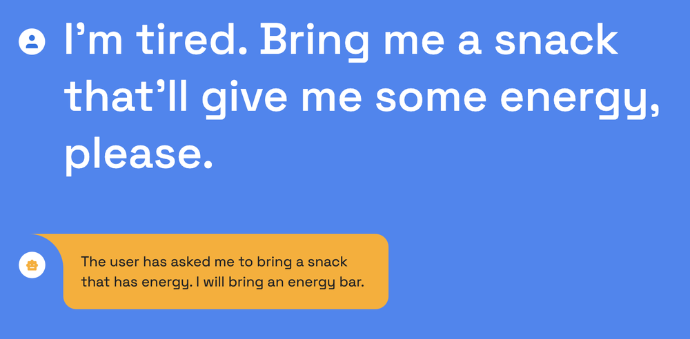
Over the last several years, we have seen significant progress in applying machine learning to robotics. However, robotic systems today are capable of executing only very short, hard-coded commands, such as “Pick up an apple,” because they tend to perform best with clear tasks and rewards. They struggle with learning to perform long-horizon tasks and reasoning about abstract goals, such as a user prompt like “I just worked out, can you get me a healthy snack?”

Meanwhile, recent progress in training language models (LMs) has led to systems that can perform a wide range of language understanding and generation tasks with impressive results. However, these language models are inherently not grounded in the physical world due to the nature of their training process: a language model generally does not interact with its environment nor observe the outcome of its responses. This can result in it generating instructions that may be illogical, impractical or unsafe for a robot to complete in a physical context. For example, when prompted with “I spilled my drink, can you help?” the language model GPT-3 responds with “You could try using a vacuum cleaner,” a suggestion that may be unsafe or impossible for the robot to execute. When asking the FLAN language model the same question, it apologizes for the spill with “I’m sorry, I didn’t mean to spill it,” which is not a very useful response. Therefore, we asked ourselves, is there an effective way to combine advanced language models with robot learning algorithms to leverage the benefits of both?

In “Do As I Can, Not As I Say: Grounding Language in Robotic Affordances”, we present a novel approach, developed in partnership with Everyday Robots, that leverages advanced language model knowledge to enable a physical agent, such as a robot, to follow high-level textual instructions for physically-grounded tasks, while grounding the language model in tasks that are feasible within a specific real-world context. We evaluate our method, which we call PaLM-SayCan, by placing robots in a real kitchen setting and giving them tasks expressed in natural language. We observe highly interpretable results for temporally-extended complex and abstract tasks, like “I just worked out, please bring me a snack and a drink to recover.” Specifically, we demonstrate that grounding the language model in the real world nearly halves errors over non-grounded baselines. We are also excited to release a robot simulation setup where the research community can test this approach.

<!–

With PaLM-SayCan, the robot acts as the language model’s “hands and eyes,” while the language model supplies high-level semantic knowledge about the task.

–>

A Dialog Between User and Robot, Facilitated by the Language Model
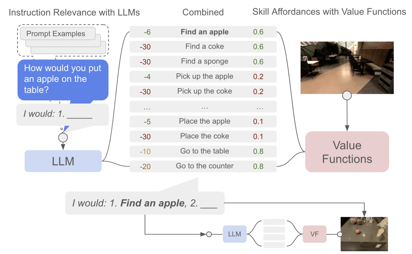
Our approach uses the knowledge contained in language models (Say) to determine and score actions that are useful towards high-level instructions. It also uses an affordance function (Can) that enables real-world-grounding and determines which actions are possible to execute in a given environment. Using the the PaLM language model, we call this PaLM-SayCan.

Our approach selects skills based on what the language model scores as useful to the high level instruction and what the affordance model scores as possible.

Our system can be seen as a dialog between the user and robot, facilitated by the language model. The user starts by giving an instruction that the language model turns into a sequence of steps for the robot to execute. This sequence is filtered using the robot’s skillset to determine the most feasible plan given its current state and environment. The model determines the probability of a specific skill successfully making progress toward completing the instruction by multiplying two probabilities: (1) task-grounding (i.e., a skill language description) and (2) world-grounding (i.e., skill feasibility in the current state).

There are additional benefits of our approach in terms of its safety and interpretability. First, by allowing the LM to score different options rather than generate the most likely output, we effectively constrain the LM to only output one of the pre-selected responses. In addition, the user can easily understand the decision making process by looking at the separate language and affordance scores, rather than a single output.

Training Policies and Value Functions
Each skill in the agent’s skillset is defined as a policy with a short language description (e.g., “pick up the can”), represented as embeddings, and an affordance function that indicates the probability of completing the skill from the robot’s current state. To learn the affordance functions, we use sparse reward functions set to 1.0 for a successful execution, and 0.0 otherwise.

We use image-based behavioral cloning (BC) to train the language-conditioned policies and temporal-difference-based (TD) reinforcement learning (RL) to train the value functions. To train the policies, we collected data from 68,000 demos performed by 10 robots over 11 months and added 12,000 successful episodes, filtered from a set of autonomous episodes of learned policies. We then learned the language conditioned value functions using MT-Opt in the Everyday Robots simulator. The simulator complements our real robot fleet with a simulated version of the skills and environment, which is transformed using RetinaGAN to reduce the simulation-to-real gap. We bootstrapped simulation policies’ performance by using demonstrations to provide initial successes, and then continuously improved RL performance with online data collection in simulation.

Given a high-level instruction, our approach combines the probabilities from the language model with the probabilities from the value function (VF) to select the next skill to perform. This process is repeated until the high-level instruction is successfully completed.

Performance on Temporally-Extended, Complex, and Abstract Instructions
To test our approach, we use robots from Everyday Robots paired with PaLM. We place the robots in a kitchen environment containing common objects and evaluate them on 101 instructions to test their performance across various robot and environment states, instruction language complexity and time horizon. Specifically, these instructions were designed to showcase the ambiguity and complexity of language rather than to provide simple, imperative queries, enabling queries such as “I just worked out, how would you bring me a snack and a drink to recover?” instead of “Can you bring me water and an apple?”

We use two metrics to evaluate the system’s performance: (1) the plan success rate, indicating whether the robot chose the right skills for the instruction, and (2) the execution success rate, indicating whether it performed the instruction successfully. We compare two language models, PaLM and FLAN (a smaller language model fine-tuned on instruction answering) with and without the affordance grounding as well as the underlying policies running directly with natural language (Behavioral Cloning in the table below). The results show that the system using PaLM with affordance grounding (PaLM-SayCan) chooses the correct sequence of skills 84% of the time and executes them successfully 74% of the time, reducing errors by 50% compared to FLAN and compared to PaLM without robotic grounding. This is particularly exciting because it represents the first time we can see how an improvement in language models translates to a similar improvement in robotics. This result indicates a potential future where robotics is able to ride the wave of progress that we have been observing in language models, bringing these subfields of research closer together.

<!–

–>

<!–<

–>

If you’re interested in learning more about this project from the researchers themselves, please check out the video below:

Conclusion and Future Work
We’re excited about the progress that we’ve seen with PaLM-SayCan, an interpretable and general approach to leveraging knowledge from language models that enables a robot to follow high-level textual instructions to perform physically-grounded tasks. Our experiments on a number of real-world robotic tasks demonstrate the ability to plan and complete long-horizon, abstract, natural language instructions at a high success rate. We believe that PaLM-SayCan’s interpretability allows for safe real-world user interaction with robots. As we explore future directions for this work, we hope to better understand how information gained via the robot’s real-world experience could be leveraged to improve the language model and to what extent natural language is the right ontology for programming robots. We have open-sourced a robot simulation setup, which we hope will provide researchers with a valuable resource for future research that combines robotic learning with advanced language models. The research community can visit the project’s GitHub page and website to learn more.

Acknowledgements
We’d like to thank our coauthors Michael Ahn, Anthony Brohan, Noah Brown, Yevgen Chebotar, Omar Cortes, Byron David, Chelsea Finn, Kelly Fu, Keerthana Gopalakrishnan, Alex Herzog, Daniel Ho, Jasmine Hsu, Julian Ibarz, Alex Irpan, Eric Jang, Rosario Jauregui Ruano, Kyle Jeffrey, Sally Jesmonth, Nikhil J Joshi, Ryan Julian, Dmitry Kalashnikov, Yuheng Kuang, Kuang-Huei Lee, Sergey Levine, Yao Lu, Linda Luu, Carolina Parada, Peter Pastor, Jornell Quiambao, Kanishka Rao, Jarek Rettinghouse, Diego Reyes, Pierre Sermanet, Nicolas Sievers, Clayton Tan, Alexander Toshev, Vincent Vanhoucke, Fei Xia, Ted Xiao, Peng Xu, Sichun Xu, Mengyuan Yan, and Andy Zeng. We’d also like to thank Yunfei Bai, Matt Bennice, Maarten Bosma, Justin Boyd, Bill Byrne, Kendra Byrne, Noah Constant, Pete Florence, Laura Graesser, Rico Jonschkowski, Daniel Kappler, Hugo Larochelle, Benjamin Lee, Adrian Li, Suraj Nair, Krista Reymann, Jeff Seto, Dhruv Shah, Ian Storz, Razvan Surdulescu, and Vincent Zhao for their help and support in various aspects of the project. And we’d like to thank Tom Small for creating many of the animations in this post.

Read More

Read More

Posted by Rolf Jagerman and Honglei Zhuang, Software Engineers, Google Research

Ranking is a core problem across a variety of domains, such as search engines, recommendation systems, or question answering. As such, researchers often utilize learning-to-rank (LTR), a set of supervised machine learning techniques that optimize for the utility of an entire list of items (rather than a single item at a time). A noticeable recent focus is on combining LTR with deep learning. Existing libraries, most notably TF-Ranking, offer researchers and practitioners the necessary tools to use LTR in their work. However, none of the existing LTR libraries work natively with JAX, a new machine learning framework that provides an extensible system of function transformations that compose: automatic differentiation, JIT-compilation to GPU/TPU devices and more.

Today, we are excited to introduce Rax, a library for LTR in the JAX ecosystem. Rax brings decades of LTR research to the JAX ecosystem, making it possible to apply JAX to a variety of ranking problems and combine ranking techniques with recent advances in deep learning built upon JAX (e.g., T5X). Rax provides state-of-the-art ranking losses, a number of standard ranking metrics, and a set of function transformations to enable ranking metric optimization. All this functionality is provided with a well-documented and easy to use API that will look and feel familiar to JAX users. Please check out our paper for more technical details.

Learning-to-Rank Using Rax
Rax is designed to solve LTR problems. To this end, Rax provides loss and metric functions that operate on batches of lists, not batches of individual data points as is common in other machine learning problems. An example of such a list is the multiple potential results from a search engine query. The figure below illustrates how tools from Rax can be used to train neural networks on ranking tasks. In this example, the green items (B, F) are very relevant, the yellow items (C, E) are somewhat relevant and the red items (A, D) are not relevant. A neural network is used to predict a relevancy score for each item, then these items are sorted by these scores to produce a ranking. A Rax ranking loss incorporates the entire list of scores to optimize the neural network, improving the overall ranking of the items. After several iterations of stochastic gradient descent, the neural network learns to score the items such that the resulting ranking is optimal: relevant items are placed at the top of the list and non-relevant items at the bottom.

Using Rax to optimize a neural network for a ranking task. The green items (B, F) are very relevant, the yellow items (C, E) are somewhat relevant and the red items (A, D) are not relevant.

Approximate Metric Optimization
The quality of a ranking is commonly evaluated using ranking metrics, e.g., the normalized discounted cumulative gain (NDCG). An important objective of LTR is to optimize a neural network so that it scores highly on ranking metrics. However, ranking metrics like NDCG can present challenges because they are often discontinuous and flat, so stochastic gradient descent cannot directly be applied to these metrics. Rax provides state-of-the-art approximation techniques that make it possible to produce differentiable surrogates to ranking metrics that permit optimization via gradient descent. The figure below illustrates the use of rax.approx_t12n, a function transformation unique to Rax, which allows for the NDCG metric to be transformed into an approximate and differentiable form.

Using an approximation technique from Rax to transform the NDCG ranking metric into a differentiable and optimizable ranking loss (approx_t12n and gumbel_t12n).

First, notice how the NDCG metric (in green) is flat and discontinuous, making it hard to optimize using stochastic gradient descent. By applying the rax.approx_t12n transformation to the metric, we obtain ApproxNDCG, an approximate metric that is now differentiable with well-defined gradients (in red). However, it potentially has many local optima — points where the loss is locally optimal, but not globally optimal — in which the training process can get stuck. When the loss encounters such a local optimum, training procedures like stochastic gradient descent will have difficulty improving the neural network further.

To overcome this, we can obtain the gumbel-version of ApproxNDCG by using the rax.gumbel_t12n transformation. This gumbel version introduces noise in the ranking scores which causes the loss to sample many different rankings that may incur a non-zero cost (in blue). This stochastic treatment may help the loss escape local optima and often is a better choice when training a neural network on a ranking metric. Rax, by design, allows the approximate and gumbel transformations to be freely used with all metrics that are offered by the library, including metrics with a top-k cutoff value, like recall or precision. In fact, it is even possible to implement your own metrics and transform them to obtain gumbel-approximate versions that permit optimization without any extra effort.

Ranking in the JAX Ecosystem
Rax is designed to integrate well in the JAX ecosystem and we prioritize interoperability with other JAX-based libraries. For example, a common workflow for researchers that use JAX is to use TensorFlow Datasets to load a dataset, Flax to build a neural network, and Optax to optimize the parameters of the network. Each of these libraries composes well with the others and the composition of these tools is what makes working with JAX both flexible and powerful. For researchers and practitioners of ranking systems, the JAX ecosystem was previously missing LTR functionality, and Rax fills this gap by providing a collection of ranking losses and metrics. We have carefully constructed Rax to function natively with standard JAX transformations such as jax.jit and jax.grad and various libraries like Flax and Optax. This means that users can freely use their favorite JAX and Rax tools together.

Ranking with T5
While giant language models such as T5 have shown great performance on natural language tasks, how to leverage ranking losses to improve their performance on ranking tasks, such as search or question answering, is under-explored. With Rax, it is possible to fully tap this potential. Rax is written as a JAX-first library, thus it is easy to integrate it with other JAX libraries. Since T5X is an implementation of T5 in the JAX ecosystem, Rax can work with it seamlessly.

To this end, we have an example that demonstrates how Rax can be used in T5X. By incorporating ranking losses and metrics, it is now possible to fine-tune T5 for ranking problems, and our results indicate that enhancing T5 with ranking losses can offer significant performance improvements. For example, on the MS-MARCO QNA v2.1 benchmark we are able to achieve a +1.2% NDCG and +1.7% MRR by fine-tuning a T5-Base model using the Rax listwise softmax cross-entropy loss instead of a pointwise sigmoid cross-entropy loss.

Fine-tuning a T5-Base model on MS-MARCO QNA v2.1 with a ranking loss (softmax, in blue) versus a non-ranking loss (pointwise sigmoid, in red).

Conclusion
Overall, Rax is a new addition to the growing ecosystem of JAX libraries. Rax is entirely open source and available to everyone at github.com/google/rax. More technical details can also be found in our paper. We encourage everyone to explore the examples included in the github repository: (1) optimizing a neural network with Flax and Optax, (2) comparing different approximate metric optimization techniques, and (3) how to integrate Rax with T5X.

Acknowledgements
Many collaborators within Google made this project possible: Xuanhui Wang, Zhen Qin, Le Yan, Rama Kumar Pasumarthi, Michael Bendersky, Marc Najork, Fernando Diaz, Ryan Doherty, Afroz Mohiuddin, and Samer Hassan.

Read More

Posted by AJ Piergiovanni and Anelia Angelova, Research Scientists, Google Research, Brain Team

Video is an ubiquitous source of media content that touches on many aspects of people’s day-to-day lives. Increasingly, real-world video applications, such as video captioning, video content analysis, and video question-answering (VideoQA), rely on models that can connect video content with text or natural language. VideoQA is particularly challenging, however, as it requires grasping both semantic information, such as objects in a scene, as well as temporal information, e.g., how things move and interact, both of which must be taken in the context of a natural-language question that holds specific intent. In addition, because videos have many frames, processing all of them to learn spatio-temporal information can be computationally expensive. Nonetheless, understanding all this information enables models to answer complex questions — for example, in the video below, a question about the second ingredient poured in the bowl requires identifying objects (the ingredients), actions (pouring), and temporal ordering (second).

An example input question for the VideoQA task “What is the second ingredient poured into the bowl?” which requires deeper understanding of both the visual and text inputs. The video is an example from the 50 Salads dataset, used under the Creative Commons license.

To address this, in “Video Question Answering with Iterative Video-Text Co-Tokenization”, we introduce a new approach to video-text learning called iterative co-tokenization, which is able to efficiently fuse spatial, temporal and language information for VideoQA. This approach is multi-stream, processing different scale videos with independent backbone models for each to produce video representations that capture different features, e.g., those of high spatial resolution or long temporal durations. The model then applies the co-tokenization module to learn efficient representations from fusing the video streams with the text. This model is highly efficient, using only 67 giga-FLOPs (GFLOPs), which is at least 50% fewer than previous approaches, while giving better performance than alternative state-of-the-art models.

Video-Text Iterative Co-tokenization
The main goal of the model is to produce features from both videos and text (i.e., the user question), jointly allowing their corresponding inputs to interact. A second goal is to do so in an efficient manner, which is highly important for videos since they contain tens to hundreds of frames as input.

The model learns to tokenize the joint video-language inputs into a smaller set of tokens that jointly and efficiently represent both modalities. When tokenizing, we use both modalities to produce a joint compact representation, which is fed to a transformer layer to produce the next level representation. A challenge here, which is also typical in cross-modal learning, is that often the video frame does not correspond directly to the associated text. We address this by adding two learnable linear layers which unify the visual and text feature dimensions before tokenization. This way we enable both video and text to condition how video tokens are learned.

Moreover, a single tokenization step does not allow for further interaction between the two modalities. For that, we use this new feature representation to interact with the video input features and produce another set of tokenized features, which are then fed into the next transformer layer. This iterative process allows the creation of new features, or tokens, which represent a continual refinement of the joint representation from both modalities. At the last step the features are input to a decoder that generates the text output.

As customarily done for VideoQA, we pre-train the model before fine-tuning it on the individual VideoQA datasets. In this work we use the videos automatically annotated with text based on speech recognition, using the HowTo100M dataset instead of pre-training on a large VideoQA dataset. This weaker pre-training data still enables our model to learn video-text features.

Visualization of the video-text iterative co-tokenization approach. Multi-stream video inputs, which are versions of the same video input (e.g., a high resolution, low frame-rate video and a low resolution, high frame-rate video), are efficiently fused together with the text input to produce a text-based answer by the decoder. Instead of processing the inputs directly, the video-text iterative co-tokenization model learns a reduced number of useful tokens from the fused video-language inputs. This process is done iteratively, allowing the current feature tokenization to affect the selection of tokens at the next iteration, thus refining the selection.

Efficient Video Question-Answering
We apply the video-language iterative co-tokenization algorithm to three main VideoQA benchmarks, MSRVTT-QA, MSVD-QA and IVQA, and demonstrate that this approach achieves better results than other state-of-the-art models, while having a modest size. Furthermore, iterative co-tokenization learning yields significant compute savings for video-text learning tasks. The method uses only 67 giga-FLOPs (GFLOPS), which is one sixth the 360 GFLOPS needed when using the popular 3D-ResNet video model jointly with text and is more than twice as efficient as the X3D model. This is all the while producing highly accurate results, outperforming state-of-the-art methods.

Comparison of our iterative co-tokenization approach to previous methods such as MERLOT and VQA-T, as well as, baselines using single ResNet-3D or X3D-XL.

Multi-stream Video Inputs
For VideoQA, or any of a number of other tasks that involve video inputs, we find that multi-stream input is important to more accurately answer questions about both spatial and temporal relationships. Our approach utilizes three video streams at different resolutions and frame-rates: a low-resolution high frame-rate, input video stream (with 32 frames-per-second and spatial resolution 64×64, which we denote as 32x64x64); a high-resolution, low frame-rate video (8x224x224); and one in-between (16x112x112). Despite the apparently more voluminous information to process with three streams, we obtain very efficient models due to the iterative co-tokenization approach. At the same time these additional streams allow extraction of the most pertinent information. For example, as shown in the figure below, questions related to a specific activity in time will produce higher activations in the smaller resolution but high frame-rate video input, whereas questions related to the general activity can be answered from the high resolution input with very few frames. Another benefit of this algorithm is that the tokenization changes depending on the questions asked.

Visualization of the attention maps learned per layer during the video-text co-tokenization. The attention maps differ depending on the question asked for the same video. For example, if the question is related to the general activity (e.g., surfing in the figure above), then the attention maps of the higher resolution low frame-rate inputs are more active and seem to consider more global information. Whereas if the question is more specific, e.g., asking about what happens after an event, the feature maps are more localized and tend to be active in the high frame-rate video input. Furthermore, we see that the low-resolution, high-frame rate video inputs provide more information related to activities in the video.

Conclusion
We present a new approach to video-language learning that focuses on joint learning across video-text modalities. We address the important and challenging task of video question-answering. Our approach is both highly efficient and accurate, outperforming current state-of-the-art models, despite being more efficient. Our approach results in modest model sizes and can gain further improvements with larger models and data. We hope this work provokes more research in vision-language learning to enable more seamless interaction with vision-based media.

Acknowledgements
This work is conducted by AJ Pierviovanni, Kairo Morton, Weicheng Kuo, Michael Ryoo and Anelia Angelova. We thank our collaborators in this research, and Soravit Changpinyo for valuable comments and suggestions, and Claire Cui for suggestions and support. We also thank Tom Small for visualizations.

Read More

Posted by Bingyi Cao, Software Engineer, Google Research, and Mário Lipovský, Software Engineer, Google Lens

Computer vision models see daily application for a wide variety of tasks, ranging from object recognition to image-based 3D object reconstruction. One challenging type of computer vision problem is instance-level recognition (ILR) — given an image of an object, the task is to not only determine the generic category of an object (e.g., an arch), but also the specific instance of the object (”Arc de Triomphe de l’Étoile, Paris, France”).

Previously, ILR was tackled using deep learning approaches. First, a large set of images was collected. Then a deep model was trained to embed each image into a high-dimensional space where similar images have similar representations. Finally, the representation was used to solve the ILR tasks related to classification (e.g., with a shallow classifier trained on top of the embedding) or retrieval (e.g., with a nearest neighbor search in the embedding space).

Since there are many different object domains in the world, e.g., landmarks, products, or artworks, capturing all of them in a single dataset and training a model that can distinguish between them is quite a challenging task. To decrease the complexity of the problem to a manageable level, the focus of research so far has been to solve ILR for a single domain at a time. To advance the research in this area, we hosted multiple Kaggle competitions focused on the recognition and retrieval of landmark images. In 2020, Amazon joined the effort and we moved beyond the landmark domain and expanded to the domains of artwork and product instance recognition. The next step is to generalize the ILR task to multiple domains.

To this end, we’re excited to announce the Google Universal Image Embedding Challenge, hosted by Kaggle in collaboration with Google Research and Google Lens. In this challenge, we ask participants to build a single universal image embedding model capable of representing objects from multiple domains at the instance level. We believe that this is the key for real-world visual search applications, such as augmenting cultural exhibits in a museum, organizing photo collections, visual commerce and more.

Images1 of object instances from some domains represented in the dataset: apparel and accessories, furniture and home goods, toys, cars, landmarks, dishes, artwork and illustrations.

Degrees of Variation in Different Domains
To represent objects from a large number of domains, we require one model to learn many domain-specific subtasks (e.g., filtering different kinds of noise or focusing on a specific detail), which can only be learned from a semantically and visually diverse collection of images. Addressing each degree of variation proposes a new challenge for both image collection and model training.

The first sort of variation comes from the fact that while some domains contain unique objects in the world (landmarks, artwork, etc.), others contain objects that may have many copies (clothing, furniture, packaged goods, food, etc.). Because a landmark is always placed at the same location, the surrounding context may be useful for recognition. In contrast, a product, say a phone, even of a specific model and color, may have millions of physical instances and thus appear in many surrounding contexts.

Another challenge comes from the fact that a single object may appear different depending on the point of view, lighting conditions, occlusion or deformations (e.g., a dress worn on a person may look very different than on a hanger). In order for a model to learn invariance to all of these visual modes, all of them should be captured by the training data.

Additionally, similarities between objects differ across domains. For example, in order for a representation to be useful in the product domain, it must be able to distinguish very fine-grained details between similarly looking products belonging to two different brands. In the domain of food, however, the same dish (e.g., spaghetti bolognese) cooked by two chefs may look quite different, but the ability of the model to distinguish spaghetti bolognese from other dishes may be sufficient for the model to be useful. Additionally, a vision model of high quality should assign similar representations to more visually similar renditions of a dish.

<!–

–><!–

–>

Domain			Landmark			Apparel
Image
Instance Name			Empire State Building2			Cycling jerseys with Android logo3
Which physical objects belong to the instance class?			Single instance in the world			Many physical instances; may differ in size or pattern (e.g., a patterned cloth cut differently)
What are the possible views of the object?			Appearance variation only based on capture conditions (e.g., illumination or viewpoint); limited number of common external views; possibility of many internal views			Deformable appearance (e.g., worn or not); limited number of common views: front, back, side
What are the surroundings and are they useful for recognition?			Surrounding context does not vary much other than daily and yearly cycles; may be useful for verifying the object of interest			Surrounding context can change dramatically due to difference in environment, additional pieces of clothing, or accessories partially occluding clothing of interest (e.g., a jacket or a scarf)
What may be tricky cases that do not belong to the instance class?			Replicas of landmarks (e.g., Eiffel Tower in Las Vegas), souvenirs			Same piece of apparel of different material or different color; visually very similar pieces with a small distinguishing detail (e.g., a small brand logo); different pieces of apparel worn by the same model

Learning Multi-domain Representations
After a collection of images covering a variety of domains is created, the next challenge is to train a single, universal model. Some features and tasks, such as representing color, are useful across many domains, and thus adding training data from any domain will likely help the model improve at distinguishing colors. Other features may be more specific to selected domains, thus adding more training data from other domains may deteriorate the model’s performance. For example, while for 2D artwork it may be very useful for the model to learn to find near duplicates, this may deteriorate the performance on clothing, where deformed and occluded instances need to be recognized.

The large variety of possible input objects and tasks that need to be learned require novel approaches for selecting, augmenting, cleaning and weighing the training data. New approaches for model training and tuning, and even novel architectures may be required.

Universal Image Embedding Challenge
To help motivate the research community to address these challenges, we are hosting the Google Universal Image Embedding Challenge. The challenge was launched on Kaggle in July and will be open until October, with cash prizes totaling $50k. The winning teams will be invited to present their methods at the Instance-Level Recognition workshop at ECCV 2022.

Participants will be evaluated on a retrieval task on a dataset of ~5,000 test query images and ~200,000 index images, from which similar images are retrieved. In contrast to ImageNet, which includes categorical labels, the images in this dataset are labeled at the instance level.

The evaluation data for the challenge is composed of images from the following domains: apparel and accessories, packaged goods, furniture and home goods, toys, cars, landmarks, storefronts, dishes, artwork, memes and illustrations.

Distribution of domains of query images.

We invite researchers and machine learning enthusiasts to participate in the Google Universal Image Embedding Challenge and join the Instance-Level Recognition workshop at ECCV 2022. We hope the challenge and the workshop will advance state-of-the-art techniques on multi-domain representations.

Acknowledgement
The core contributors to this project are Andre Araujo, Boris Bluntschli, Bingyi Cao, Kaifeng Chen, Mário Lipovský, Grzegorz Makosa, Mojtaba Seyedhosseini and Pelin Dogan Schönberger. We would like to thank Sohier Dane, Will Cukierski and Maggie Demkin for their help organizing the Kaggle challenge, as well as our ECCV workshop co-organizers Tobias Weyand, Bohyung Han, Shih-Fu Chang, Ondrej Chum, Torsten Sattler, Giorgos Tolias, Xu Zhang, Noa Garcia, Guangxing Han, Pradeep Natarajan and Sanqiang Zhao. Furthermore we are thankful to Igor Bonaci, Tom Duerig, Vittorio Ferrari, Victor Gomes, Futang Peng and Howard Zhou who gave us feedback, ideas and support at various points of this project.

¹ Image credits: Chris Schrier, CC-BY; Petri Krohn, GNU Free Documentation License; Drazen Nesic, CC0; Marco Verch Professional Photographer, CCBY; Grendelkhan, CCBY; Bobby Mikul, CC0; Vincent Van Gogh, CC0; pxhere.com, CC0; Smart Home Perfected, CC-BY.  ^↩
2 Image credit: Bobby Mikul, CC0.  ^↩
3 Image credit: Chris Schrier, CC-BY.  ^↩

Read More

Posted by Qifei Wang, Senior Software Engineer, and Feng Yang, Senior Staff Software Engineer, Google Research

Deep learning models for visual tasks (e.g., image classification) are usually trained end-to-end with data from a single visual domain (e.g., natural images or computer generated images). Typically, an application that completes visual tasks for multiple domains would need to build multiple models for each individual domain, train them independently (meaning no data is shared between domains), and then at inference time each model would process domain-specific input data. However, early layers between these models generate similar features, even for different domains, so it can be more efficient — decreasing latency and power consumption, lower memory overhead to store parameters of each model — to jointly train multiple domains, an approach referred to as multi-domain learning (MDL). Moreover, an MDL model can also outperform single domain models due to positive knowledge transfer, which is when additional training on one domain actually improves performance for another. The opposite, negative knowledge transfer, can also occur, depending on the approach and specific combination of domains involved. While previous work on MDL has proven the effectiveness of jointly learning tasks across multiple domains, it involved a hand-crafted model architecture that is inefficient to apply to other work.

In “Multi-path Neural Networks for On-device Multi-domain Visual Classification”, we propose a general MDL model that can: 1) achieve high accuracy efficiently (keeping the number of parameters and FLOPS low), 2) learn to enhance positive knowledge transfer while mitigating negative transfer, and 3) effectively optimize the joint model while handling various domain-specific difficulties. As such, we propose a multi-path neural architecture search (MPNAS) approach to build a unified model with heterogeneous network architecture for multiple domains. MPNAS extends the efficient neural architecture search (NAS) approach from single path search to multi-path search by finding an optimal path for each domain jointly. Also, we introduce a new loss function, called adaptive balanced domain prioritization (ABDP) that adapts to domain-specific difficulties to help train the model efficiently. The resulting MPNAS approach is efficient and scalable; the resulting model maintains performance while reducing the model size and FLOPS by 78% and 32%, respectively, compared to a single-domain approach.

Multi-Path Neural Architecture Search
To encourage positive knowledge transfer and avoid negative transfer, traditional solutions build an MDL model so that domains share most of the layers that learn the shared features across domains (called feature extraction), then have a few domain-specific layers on top. However, such a homogenous approach to feature extraction cannot handle domains with significantly different features (e.g., objects in natural images and art paintings). On the other hand, handcrafting a unified heterogeneous architecture for each MDL model is time-consuming and requires domain-specific knowledge.

NAS is a powerful paradigm for automatically designing deep learning architectures. It defines a search space, made up of various potential building blocks that could be part of the final model. The search algorithm finds the best candidate architecture from the search space that optimizes the model objectives, e.g., classification accuracy. Recent NAS approaches (e.g., TuNAS) have meaningfully improved search efficiency by using end-to-end path sampling, which enables us to scale NAS from single domains to MDL.

Inspired by TuNAS, MPNAS builds the MDL model architecture in two stages: search and training. In the search stage, to find an optimal path for each domain jointly, MPNAS creates an individual reinforcement learning (RL) controller for each domain, which samples an end-to-end path (from input layer to output layer) from the supernetwork (i.e., the superset of all the possible subnetworks between the candidate nodes defined by the search space). Over multiple iterations, all the RL controllers update the path to optimize the RL rewards across all domains. At the end of the search stage, we obtain a subnetwork for each domain. Finally, all the subnetworks are combined to build a heterogeneous architecture for the MDL model, shown below.

Since the subnetwork for each domain is searched independently, the building block in each layer can be shared by multiple domains (i.e., dark gray nodes), used by a single domain (i.e., light gray nodes), or not used by any subnetwork (i.e., dotted nodes). The path for each domain can also skip any layer during search. Given the subnetwork can freely select which blocks to use along the path in a way that optimizes performance (rather than, e.g., arbitrarily designating which layers are homogenous and which are domain-specific), the output network is both heterogeneous and efficient.

Example architecture searched by MPNAS. Dashed paths represent all the possible subnetworks. Solid paths represent the selected subnetworks for each domain (highlighted in different colors). Nodes in each layer represent the candidate building blocks defined by the search space.

The figure below demonstrates the searched architecture of two visual domains among the ten domains of the Visual Domain Decathlon challenge. One can see that the subnetwork of these two highly related domains (one red, the other green) share a majority of building blocks from their overlapping paths, but there are still some differences.

Architecture blocks of two domains (ImageNet and Describable Textures) among the ten domains of the Visual Domain Decathlon challenge. Red and green path represents the subnetwork of ImageNet and Describable Textures, respectively. Dark pink nodes represent the blocks shared by multiple domains. Light pink nodes represent the blocks used by each path. The model is built based on MobileNet V3-like search space. The “dwb” block in the figure represents the dwbottleneck block. The “zero” block in the figure indicates the subnetwork skips that block.

Below we show the path similarity between domains among the ten domains of the Visual Domain Decathlon challenge. The similarity is measured by the Jaccard similarity score between the subnetworks of each domain, where higher means the paths are more similar. As one might expect, domains that are more similar share more nodes in the paths generated by MPNAS, which is also a signal of strong positive knowledge transfer. For example, the paths for similar domains (like ImageNet, CIFAR-100, and VGG Flower, which all include objects in natural images) have high scores, while the paths for dissimilar domains (like Daimler Pedestrian Classification and UCF101 Dynamic Images, which include pedestrians in grayscale images and human activity in natural color images, respectively) have low scores.

Confusion matrix for the Jaccard similarity score between the paths for the ten domains. Score value ranges from 0 to 1. A greater value indicates two paths share more nodes.

Training a Heterogeneous Multi-domain Model
In the second stage, the model resulting from MPNAS is trained from scratch for all domains. For this to work, it is necessary to define a unified objective function for all the domains. To successfully handle a large variety of domains, we designed an algorithm that adapts throughout the learning process such that losses are balanced across domains, called adaptive balanced domain prioritization (ABDP).

Below we show the accuracy, model size, and FLOPS of the model trained in different settings. We compare MPNAS to three other approaches:

• Domain independent NAS: Searching and training a model for each domain separately.
• Single path multi-head: Using a pre-trained model as a shared backbone for all domains with separated classification heads for each domain.
• Multi-head NAS: Searching a unified backbone architecture for all domains with separated classification heads for each domain.

From the results, we can observe that domain independent NAS requires building a bundle of models for each domain, resulting in a large model size. Although single path multi-head and multi-head NAS can reduce the model size and FLOPS significantly, forcing the domains to share the same backbone introduces negative knowledge transfer, decreasing overall accuracy.

MPNAS can build a small and efficient model while still maintaining high overall accuracy. The average accuracy of MPNAS is even 1.9% higher than the domain independent NAS approach since the model enables positive knowledge transfer. The figure below compares per domain top-1 accuracy of these approaches.

Top-1 accuracy of each Visual Decathlon domain.

Our evaluation shows that top-1 accuracy is improved from 69.96% to 71.78% (delta: +1.81%) by using ABDP as part of the search and training stages.

Top-1 accuracy for each Visual Decathlon domain trained by MPNAS with and without ABDP.

Future Work
We find MPNAS is an efficient solution to build a heterogeneous network to address the data imbalance, domain diversity, negative transfer, domain scalability, and large search space of possible parameter sharing strategies in MDL. By using a MobileNet-like search space, the resulting model is also mobile friendly. We are continuing to extend MPNAS for multi-task learning for tasks that are not compatible with existing search algorithms and hope others might use MPNAS to build a unified multi-domain model.

Acknowledgements
This work is made possible through a collaboration spanning several teams across Google. We’d like to acknowledge contributions from Junjie Ke, Joshua Greaves, Grace Chu, Ramin Mehran, Gabriel Bender, Xuhui Jia, Brendan Jou, Yukun Zhu, Luciano Sbaiz, Alec Go, Andrew Howard, Jeff Gilbert, Peyman Milanfar, and Ming-Tsuan Yang.

Read More

Posted by Arun Kandoor, Software Engineer, Google Research

The increasing demand for machine learning (ML) model inference on-device (for mobile devices, tablets, etc.) is driven by the rise of compute-intensive applications, the need to keep certain data on device for privacy and security reasons, and the desire to provide services when a network connection may not be available. However, on-device inference introduces a myriad of challenges, ranging from modeling to platform support requirements. These challenges relate to how different architectures are designed to optimize memory and computation, while still trying to maintain the quality of the model. From a platform perspective, the issue is identifying operations and building on top of them in a way that can generalize well across different product use cases.

In previous research, we combined a novel technique for generating embeddings (called projection-based embeddings) with efficient architectures like QRNN (pQRNN) and proved them to be competent for a number of classification problems. Augmenting these with distillation techniques provides an additional bump in end-to-end quality. Although this is an effective approach, it is not scalable to bigger and more extensive vocabularies (i.e., all possible Unicode or word tokens that can be fed to the model). Additionally, the output from the projection operation itself doesn’t contain trainable weights to take advantage of pre-training the model.

Token-free models presented in ByT5 are a good starting point for on-device modeling that can address pre-training and scalability issues without the need to increase the size of the model. This is possible because these approaches treat text inputs as a stream of bytes (each byte has a value that ranges from 0 to 255) that can reduce the vocabulary size for the embedding tables from ~30,000 to 256. Although ByT5 presents a compelling alternative for on-device modeling, going from word-level representation to byte stream representation increases the sequence lengths linearly; with an average word length of four characters and a single character having up to four bytes, the byte sequence length increases proportionally to the word length. This can lead to a significant increase in inference latency and computational costs.

We address this problem by developing and releasing three novel byte-stream sequence models for the SeqFlowLite library (ByteQRNN, ByteTransformer and ByteFunnelTransformer), all of which can be pre-trained on unsupervised data and can be fine-tuned for specific tasks. These models leverage recent innovations introduced by Charformer, including a fast character Transformer-based model that uses a gradient-based subword tokenization (GBST) approach to operate directly at the byte level, as well as a “soft” tokenization approach, which allows us to learn token boundaries and reduce sequence lengths. In this post, we focus on ByteQRNN and demonstrate that the performance of a pre-trained ByteQRNN model is comparable to BERT, despite being 300x smaller.

Sequence Model Architecture
We leverage pQRNN, ByT5 and Charformer along with platform optimizations, such as in-training quantization (which tracks minimum and maximum float values for model activations and weights for quantizing the inference model) that reduces model sizes by one-fourth, to develop an end-to-end model called ByteQRNN (shown below). First, we use a ByteSplitter operation to split the input string into a byte stream and feed it to a smaller embedding table that has a vocabulary size of 259 (256 + 3 additional meta tokens).

The output from the embedding layer is fed to the GBST layer, which is equipped with in-training quantization and combines byte-level representations with the efficiency of subword tokenization while enabling end-to-end learning of latent subwords. We “soft” tokenize the byte stream sequences by enumerating and combining each subword block length with scores (computed with a quantized dense layer) at each strided token position (i.e., at token positions that are selected at regular intervals). Next, we downsample the byte stream to manageable sequence length and feed it to the encoder layer.

The output from the GBST layer can be downsampled to a lower sequence length for efficient encoder computation or can be used by an encoder, like Funnel Transformer, which pools the query length and reduces the self-attention computation to create the ByteFunnelTransformer model. The encoder in the end-to-end model can be replaced with any other encoder layer, such as the Transformer from the SeqFlowLite library, to create a ByteTransformer model.

A diagram of a generic end-to-end sequence model using byte stream input. The ByteQRNN model uses a QRNN encoder from the SeqFlowLite library.

In addition to the input embeddings (i.e., the output from the embedding layer described above), we go a step further to build an effective sequence-to-sequence (seq2seq) model. We do so by taking ByteQRNN and adding a Transformer-based decoder model along with a quantized beam search (or tree exploration) to go with it. The quantized beam search module reduces the inference latency when generating decoder outputs by computing the most likely beams (i.e., possible output sequences) using the logarithmic sum of previous and current probabilities and returns the resulting top beams. Here the system uses a more efficient 8-bit integer (uint8) format, compared to a typical single-precision floating-point format (float32) model.

The decoder Transformer model uses a merged attention sublayer (MAtt) to reduce the complexity of the decoder self-attention from quadratic to linear, thereby lowering the end-to-end latency. For each decoding step, MAtt uses a fixed-size cache for decoder self-attention compared to the increasing cache size of a traditional transformer decoder. The following figure illustrates how the beam search module interacts with the decoder layer to generate output tokens on-device using an edge device (e.g., mobile phones, tablets, etc.).

A comparison of cloud server decoding and on-device (edge device) implementation. Left: Cloud server beam search employs a Transformer-based decoder model with quadratic time self-attention in float32, which has an increasing cache size for each decoding step. Right: The edge device implementation employs a quantized beam search module along with a fixed-size cache and a linear time self-attention computation.

Evaluation
After developing ByteQRNN, we evaluate its performance on the civil_comments dataset using the area under the curve (AUC) metric and compare it to a pre-trained ByteQRNN and BERT (shown below). We demonstrate that the fine-tuned ByteQRNN improves the overall quality and brings its performance closer to the BERT models, despite being 300x smaller. Since SeqFlowLite models support in-training quantization that reduces model sizes by one-fourth, the resulting models scale well to low-compute devices. We chose multilingual data sources that related to the task for pre-training both BERT and byte stream models to achieve the best possible performance.

Comparison of ByteQRNN with fine-tuned ByteQRNN and BERT on the civil_comments dataset.

Conclusion
Following up on our previous work with pQRNN, we evaluate byte stream models for on-device use to enable pre-training and thereby improve model performance for on-device deployment. We present an evaluation for ByteQRNN with and without pre-training and demonstrate that the performance of the pre-trained ByteQRNN is comparable to BERT, despite being 300x smaller. In addition to ByteQRNN, we are also releasing ByteTransformer and ByteFunnelTransformer, two models which use different encoders, along with the merged attention decoder model and the beam search driver to run the inference through the SeqFlowLite library. We hope these models will provide researchers and product developers with valuable resources for future on-device deployments.

Acknowledgements
We would like to thank Khoa Trinh, Jeongwoo Ko, Peter Young and Yicheng Fan for helping with open-sourcing and evaluating the model. Thanks to Prabhu Kaliamoorthi for all the brainstorming and ideation. Thanks to Vinh Tran, Jai Gupta and Yi Tay for their help with pre-training byte stream models. Thanks to Ruoxin Sang, Haoyu Zhang, Ce Zheng, Chuanhao Zhuge and Jieying Luo for helping with the TPU training. Many thanks to Erik Vee, Ravi Kumar and the Learn2Compress leadership for sponsoring the project and their support and encouragement. Finally, we would like to thank Tom Small for the animated figure used in this post.

Read More

Posted by Ehsan Amid, Research Scientist, and Rohan Anil, Principal Engineer, Google Research, Brain Team

While model design and training data are key ingredients in a deep neural network’s (DNN’s) success, less-often discussed is the specific optimization method used for updating the model parameters (weights). Training DNNs involves minimizing a loss function that measures the discrepancy between the ground truth labels and the model’s predictions. Training is carried out by backpropagation, which adjusts the model weights via gradient descent steps. Gradient descent, in turn, updates the weights by using the gradient (i.e., derivative) of the loss with respect to the weights.

The simplest weight update corresponds to stochastic gradient descent, which, in every step, moves the weights in the negative direction with respect to the gradients (with an appropriate step size, a.k.a. the learning rate). More advanced optimization methods modify the direction of the negative gradient before updating the weights by using information from the past steps and/or the local properties (such as the curvature information) of the loss function around the current weights. For instance, a momentum optimizer encourages moving along the average direction of past updates, and the AdaGrad optimizer scales each coordinate based on the past gradients. These optimizers are commonly known as first-order methods since they generally modify the update direction using only information from the first-order derivative (i.e., gradient). More importantly, the components of the weight parameters are treated independently from each other.

More advanced optimization, such as Shampoo and K-FAC, capture the correlations between gradients of parameters and have been shown to improve convergence, reducing the number of iterations and improving the quality of the solution. These methods capture information about the local changes of the derivatives of the loss, i.e., changes in gradients. Using this additional information, higher-order optimizers can discover much more efficient update directions for training models by taking into account the correlations between different groups of parameters. On the downside, calculating higher-order update directions is computationally more expensive than first-order updates. The operation uses more memory for storing statistics and involves matrix inversion, thus hindering the applicability of higher-order optimizers in practice.

In “LocoProp: Enhancing BackProp via Local Loss Optimization”, we introduce a new framework for training DNN models. Our new framework, LocoProp, conceives neural networks as a modular composition of layers. Generally, each layer in a neural network applies a linear transformation on its inputs, followed by a non-linear activation function. In the new construction, each layer is allotted its own weight regularizer, output target, and loss function. The loss function of each layer is designed to match the activation function of the layer. Using this formulation, training minimizes the local losses for a given mini-batch of examples, iteratively and in parallel across layers. Our method performs multiple local updates per batch of examples using a first-order optimizer (like RMSProp), which avoids computationally expensive operations such as the matrix inversions required for higher-order optimizers. However, we show that the combined local updates look rather like a higher-order update. Empirically, we show that LocoProp outperforms first-order methods on a deep autoencoder benchmark and performs comparably to higher-order optimizers, such as Shampoo and K-FAC, without the high memory and computation requirements.

Method
Neural networks are generally viewed as composite functions that transform model inputs into output representations, layer by layer. LocoProp adopts this view while decomposing the network into layers. In particular, instead of updating the weights of the layer to minimize the loss function at the output, LocoProp applies pre-defined local loss functions specific to each layer. For a given layer, the loss function is selected to match the activation function, e.g., a tanh loss would be selected for a layer with a tanh activation. Each layerwise loss measures the discrepancy between the layer’s output (for a given mini-batch of examples) and a notion of a target output for that layer. Additionally, a regularizer term ensures that the updated weights do not drift too far from the current values. The combined layerwise loss function (with a local target) plus regularizer is used as the new objective function for each layer.

Similar to backpropagation, LocoProp applies a forward pass to compute the activations. In the backward pass, LocoProp sets per neuron “targets” for each layer. Finally, LocoProp splits model training into independent problems across layers where several local updates can be applied to each layer’s weights in parallel.

Perhaps the simplest loss function one can think of for a layer is the squared loss. While the squared loss is a valid choice of a loss function, LocoProp takes into account the possible non-linearity of the activation functions of the layers and applies layerwise losses tailored to the activation function of each layer. This enables the model to emphasize regions at the input that are more important for the model prediction while deemphasizing the regions that do not affect the output as much. Below we show examples of tailored losses for the tanh and ReLU activation functions.

Loss functions induced by the (left) tanh and (right) ReLU activation functions. Each loss is more sensitive to the regions affecting the output prediction. For instance, ReLU loss is zero as long as both the prediction (â) and the target (a) are negative. This is because the ReLU function applied to any negative number equals zero.

After forming the objective in each layer, LocoProp updates the layer weights by repeatedly applying gradient descent steps on its objective. The update typically uses a first-order optimizer (like RMSProp). However, we show that the overall behavior of the combined updates closely resembles higher-order updates (shown below). Thus, LocoProp provides training performance close to what higher-order optimizers achieve without the high memory or computation needed for higher-order methods, such as matrix inverse operations. We show that LocoProp is a flexible framework that allows the recovery of well-known algorithms and enables the construction of new algorithms via different choices of losses, targets, and regularizers. LocoProp’s layerwise view of neural networks also allows updating the weights in parallel across layers.

Experiments
In our paper, we describe experiments on the deep autoencoder model, which is a commonly used baseline for evaluating the performance of optimization algorithms. We perform extensive tuning on multiple commonly used first-order optimizers, including SGD, SGD with momentum, AdaGrad, RMSProp, and Adam, as well as the higher-order Shampoo and K-FAC optimizers, and compare the results with LocoProp. Our findings indicate that the LocoProp method performs significantly better than first-order optimizers and is comparable to those of higher-order, while being significantly faster when run on a single GPU.

Train loss vs. number of epochs (left) and wall-clock time, i.e., the real time that passes during training, (right) for RMSProp, Shampoo, K-FAC, and LocoProp on the deep autoencoder model.

Summary and Future Directions
We introduced a new framework, called LocoProp, for optimizing deep neural networks more efficiently. LocoProp decomposes neural networks into separate layers with their own regularizer, output target, and loss function and applies local updates in parallel to minimize the local objectives. While using first-order updates for the local optimization problems, the combined updates closely resemble higher-order update directions, both theoretically and empirically.

LocoProp provides flexibility to choose the layerwise regularizers, targets, and loss functions. Thus, it allows the development of new update rules based on these choices. Our code for LocoProp is available online on GitHub. We are currently working on scaling up ideas induced by LocoProp to much larger scale models; stay tuned!

Acknowledgments
We would like to thank our co-author, Manfred K. Warmuth, for his critical contributions and inspiring vision. We would like to thank Sameer Agarwal for discussions looking at this work from a composite functions perspective, Vineet Gupta for discussions and development of Shampoo, Zachary Nado on K-FAC, Tom Small for development of the animation used in this blogpost and finally, Yonghui Wu and Zoubin Ghahramani for providing us with a nurturing research environment in the Google Brain Team.

Read More

Posted by Tuan Anh Nguyen, Google Assistant and Sourish Chaudhuri, Google Research

In natural conversations, we don’t say people’s names every time we speak to each other. Instead, we rely on contextual signaling mechanisms to initiate conversations, and eye contact is often all it takes. Google Assistant, now available in more than 95 countries and over 29 languages, has primarily relied on a hotword mechanism (“Hey Google” or “OK Google”) to help more than 700 million people every month get things done across Assistant devices. As virtual assistants become an integral part of our everyday lives, we’re developing ways to initiate conversations more naturally.

At Google I/O 2022, we announced Look and Talk, a major development in our journey to create natural and intuitive ways to interact with Google Assistant-powered home devices. This is the first multimodal, on-device Assistant feature that simultaneously analyzes audio, video, and text to determine when you are speaking to your Nest Hub Max. Using eight machine learning models together, the algorithm can differentiate intentional interactions from passing glances in order to accurately identify a user’s intent to engage with Assistant. Once within 5ft of the device, the user may simply look at the screen and talk to start interacting with the Assistant.

We developed Look and Talk in alignment with our AI Principles. It meets our strict audio and video processing requirements, and like our other camera sensing features, video never leaves the device. You can always stop, review and delete your Assistant activity at myactivity.google.com. These added layers of protection enable Look and Talk to work just for those who turn it on, while keeping your data safe.

Google Assistant relies on a number of signals to accurately determine when the user is speaking to it. On the right is a list of signals used with indicators showing when each signal is triggered based on the user’s proximity to the device and gaze direction.

Modeling Challenges
The journey of this feature began as a technical prototype built on top of models developed for academic research. Deployment at scale, however, required solving real-world challenges unique to this feature. It had to:

1. Support a range of demographic characteristics (e.g., age, skin tones).
2. Adapt to the ambient diversity of the real world, including challenging lighting (e.g., backlighting, shadow patterns) and acoustic conditions (e.g., reverberation, background noise).
3. Deal with unusual camera perspectives, since smart displays are commonly used as countertop devices and look up at the user(s), unlike the frontal faces typically used in research datasets to train models.
4. Run in real-time to ensure timely responses while processing video on-device.

The evolution of the algorithm involved experiments with approaches ranging from domain adaptation and personalization to domain-specific dataset development, field-testing and feedback, and repeated tuning of the overall algorithm.

Technology Overview
A Look and Talk interaction has three phases. In the first phase, Assistant uses visual signals to detect when a user is demonstrating an intent to engage with it and then “wakes up” to listen to their utterance. The second phase is designed to further validate and understand the user’s intent using visual and acoustic signals. If any signal in the first or second processing phases indicates that it isn’t an Assistant query, Assistant returns to standby mode. These two phases are the core Look and Talk functionality, and are discussed below. The third phase of query fulfillment is typical query flow, and is beyond the scope of this blog.

Phase One: Engaging with Assistant
The first phase of Look and Talk is designed to assess whether an enrolled user is intentionally engaging with Assistant. Look and Talk uses face detection to identify the user’s presence, filters for proximity using the detected face box size to infer distance, and then uses the existing Face Match system to determine whether they are enrolled Look and Talk users.

For an enrolled user within range, an custom eye gaze model determines whether they are looking at the device. This model estimates both the gaze angle and a binary gaze-on-camera confidence from image frames using a multi-tower convolutional neural network architecture, with one tower processing the whole face and another processing patches around the eyes. Since the device screen covers a region underneath the camera that would be natural for a user to look at, we map the gaze angle and binary gaze-on-camera prediction to the device screen area. To ensure that the final prediction is resilient to spurious individual predictions and involuntary eye blinks and saccades, we apply a smoothing function to the individual frame-based predictions to remove spurious individual predictions.

Eye-gaze prediction and post-processing overview.

We enforce stricter attention requirements before informing users that the system is ready for interaction to minimize false triggers, e.g., when a passing user briefly glances at the device. Once the user looking at the device starts speaking, we relax the attention requirement, allowing the user to naturally shift their gaze.

The final signal necessary in this processing phase checks that the Face Matched user is the active speaker. This is provided by a multimodal active speaker detection model that takes as input both video of the user’s face and the audio containing speech, and predicts whether they are speaking. A number of augmentation techniques (including RandAugment, SpecAugment, and augmenting with AudioSet sounds) helps improve prediction quality for the in-home domain, boosting end-feature performance by over 10%.The final deployed model is a quantized, hardware-accelerated TFLite model, which uses five frames of context for the visual input and 0.5 seconds for the audio input.

Active speaker detection model overview: The two-tower audiovisual model provides the “speaking” probability prediction for the face. The visual network auxiliary prediction pushes the visual network to be as good as possible on its own, improving the final multimodal prediction.

Phase Two: Assistant Starts Listening
In phase two, the system starts listening to the content of the user’s query, still entirely on-device, to further assess whether the interaction is intended for Assistant using additional signals. First, Look and Talk uses Voice Match to further ensure that the speaker is enrolled and matches the earlier Face Match signal. Then, it runs a state-of-the-art automatic speech recognition model on-device to transcribe the utterance.

The next critical processing step is the intent understanding algorithm, which predicts whether the user’s utterance was intended to be an Assistant query. This has two parts: 1) a model that analyzes the non-lexical information in the audio (i.e., pitch, speed, hesitation sounds) to determine whether the utterance sounds like an Assistant query, and 2) a text analysis model that determines whether the transcript is an Assistant request. Together, these filter out queries not intended for Assistant. It also uses contextual visual signals to determine the likelihood that the interaction was intended for Assistant.

Overview of the semantic filtering approach to determine if a user utterance is a query intended for the Assistant.

Finally, when the intent understanding model determines that the user utterance was likely meant for Assistant, Look and Talk moves into the fulfillment phase where it communicates with the Assistant server to obtain a response to the user’s intent and query text.

Performance, Personalization and UX
Each model that supports Look and Talk was evaluated and improved in isolation and then tested in the end-to-end Look and Talk system. The huge variety of ambient conditions in which Look and Talk operates necessitates the introduction of personalization parameters for algorithm robustness. By using signals obtained during the user’s hotword-based interactions, the system personalizes parameters to individual users to deliver improvements over the generalized global model. This personalization also runs entirely on-device.

Without a predefined hotword as a proxy for user intent, latency was a significant concern for Look and Talk. Often, a strong enough interaction signal does not occur until well after the user has started speaking, which can add hundreds of milliseconds of latency, and existing models for intent understanding add to this since they require complete, not partial, queries. To bridge this gap, Look and Talk completely forgoes streaming audio to the server, with transcription and intent understanding being on-device. The intent understanding models can work off of partial utterances. This results in an end-to-end latency comparable with current hotword-based systems.

The UI experience is based on user research to provide well-balanced visual feedback with high learnability. This is illustrated in the figure below.

Left: The spatial interaction diagram of a user engaging with Look and Talk. Right: The User Interface (UI) experience.

We developed a diverse video dataset with over 3,000 participants to test the feature across demographic subgroups. Modeling improvements driven by diversity in our training data improved performance for all subgroups.

Conclusion
Look and Talk represents a significant step toward making user engagement with Google Assistant as natural as possible. While this is a key milestone in our journey, we hope this will be the first of many improvements to our interaction paradigms that will continue to reimagine the Google Assistant experience responsibly. Our goal is to make getting help feel natural and easy, ultimately saving time so users can focus on what matters most.

Acknowledgements
This work involved collaborative efforts from a multidisciplinary team of software engineers, researchers, UX, and cross-functional contributors. Key contributors from Google Assistant include Alexey Galata, Alice Chuang‎, Barbara Wang, Britanie Hall, Gabriel Leblanc, Gloria McGee, Hideaki Matsui, James Zanoni, Joanna (Qiong) Huang, Krunal Shah, Kavitha Kandappan, Pedro Silva, Tanya Sinha, Tuan Nguyen, Vishal Desai, Will Truong‎, Yixing Cai‎, Yunfan Ye; from Research including Hao Wu, Joseph Roth, Sagar Savla, Sourish Chaudhuri, Susanna Ricco. Thanks to Yuan Yuan and Caroline Pantofaru for their leadership, and everyone on the Nest, Assistant, and Research teams who provided invaluable input toward the development of Look and Talk.

Read More