Posts in category: Google AI

Hanie Sedghi, Google Research and Preetum Nakkiran, Harvard University

Understanding generalization is one of the fundamental unsolved problems in deep learning. Why does optimizing a model on a finite set of training data lead to good performance on a held-out test set? This problem has been studied extensively in machine learning, with a rich history going back more than 50 years. There are now many mathematical tools that help researchers understand generalization in certain models. Unfortunately, most of these existing theories fail when applied to modern deep networks — they are both vacuous and non-predictive in realistic settings. This gap between theory and practice is largest for overparameterized models, which in theory have the capacity to overfit their train sets, but often do not in practice.

In “The Deep Bootstrap Framework: Good Online Learners are Good Offline Generalizers”, accepted at ICLR 2021, we present a new framework for approaching this problem by connecting generalization to the field of online optimization. In a typical setting, a model trains on a finite set of samples, which are reused for multiple epochs. But in online optimization, the model has access to an infinite stream of samples, and can be iteratively updated while processing this stream. In this work, we find that models that train quickly on infinite data are the same models that generalize well if they are instead trained on finite data. This connection brings new perspectives on design choices in practice, and lays a roadmap for understanding generalization from a theoretical perspective.

The Deep Bootstrap Framework
The main idea of the Deep Bootstrap framework is to compare the real world, where there is finite training data, to an “ideal world”, where there is infinite data. We define these as:

• Real World (N, T): Train a model on N train samples from a distribution, for T minibatch stochastic gradient descent (SGD) steps, re-using the same N samples in multiple epochs, as usual. This corresponds to running SGD on the empirical loss (loss on training data), and is the standard training procedure in supervised learning.

• Ideal World (T): Train the same model for T steps, but use fresh samples from the distribution in each SGD step. That is, we run the exact same training code (same optimizer, learning-rates, batch-size, etc.), but sample a fresh train set in each epoch instead of reusing samples. In this ideal world setting, with an effectively infinite “train set”, there is no difference between train error and test error.

Test soft-error for ideal world and real world during SGD iterations for ResNet-18 architecture. We see that the two errors are similar.

A priori, one might expect the real and ideal worlds may have nothing to do with each other, since in the real world the model sees a finite number of examples from the distribution while in the ideal world the model sees the whole distribution. But in practice, we found that the real and ideal models actually have similar test error.

In order to quantify this observation, we simulated an ideal world setting by creating a new dataset, which we call CIFAR-5m. We trained a generative model on CIFAR-10, which we then used to generate ~6 million images. The scale of the dataset was chosen to ensure that it is “virtually infinite” from the model’s perspective, so that the model never resamples the same data. That is, in the ideal world, the model sees an entirely fresh set of samples.

Samples from CIFAR-5m

The figure below presents the test error of several models, comparing their performance when trained on CIFAR-5m data in the real world setting (i.e., re-used data) and the ideal world (“fresh” data). The solid blue line shows a ResNet model in the real world, trained on 50K samples for 100 epochs with standard CIFAR-10 hyperparameters. The dashed blue line shows the corresponding model in the ideal world, trained on 5 million samples in a single pass. Surprisingly, these worlds have very similar test error — the model in some sense “doesn’t care” whether it sees re-used samples or fresh ones.

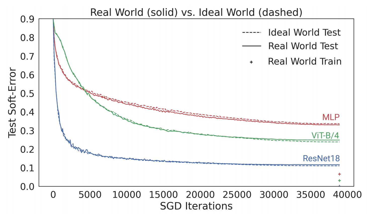
The real world model is trained on 50K samples for 100 epochs, and the ideal world model is trained on 5M samples for a single epoch. The lines show the test error vs. the number of SGD steps.

This also holds for other architectures, e.g., a Multi-Layer-Perceptron (red), a Vision Transformer (green), and across many other settings of architecture, optimizer, data distribution, and sample size. These experiments suggest a new perspective on generalization: models that optimize quickly (on infinite data), generalize well (on finite data). For example, the ResNet model generalizes better than the MLP model on finite data, but this is “because” it optimizes faster even on infinite data.

Understanding Generalization from Optimization Behavior
The key observation is that real world and ideal world models remain close, in test error, for all timesteps, until the real world converges (< 1% train error). Thus, one can study models in the real world by studying their corresponding behavior in the ideal world.

This means that the generalization of the model can be understood in terms of its optimization performance under two frameworks:

1. Online Optimization: How fast the ideal world test error decreases
2. Offline Optimization: How fast the real world train error converges

Thus, to study generalization, we can equivalently study the two terms above, which can be conceptually simpler, since they only involve optimization concerns. Based on this observation, good models and training procedures are those that (1) optimize quickly in the ideal world and (2) do not optimize too quickly in the real world.

All design choices in deep learning can be viewed through their effect on these two terms. For example, some advances like convolutions, skip-connections, and pre–training help primarily by accelerating ideal world optimization, while other advances like regularization and data-augmentation help primarily by decelerating real world optimization.

Applying the Deep Bootstrap Framework
Researchers can use the Deep Bootstrap framework to study and guide design choices in deep learning. The principle is: whenever one makes a change that affects generalization in the real world (the architecture, learning-rate, etc.), one should consider its effect on (1) the ideal world optimization of test error (faster is better) and (2) the real world optimization of train error (slower is better).

For example, pre-training is often used in practice to help generalization of models in small-data regimes. However, the reason that pre-training helps remains poorly understood. One can study this using the Deep Bootstrap framework by looking at the effect of pre-training on terms (1) and (2) above. We find that the primary effect of pre-training is to improve the ideal world optimization (1) — pre-training turns the network into a “fast learner” for online optimization. The improved generalization of pretrained models is thus almost exactly captured by their improved optimization in the ideal world. The figure below shows this for Vision-Transformers (ViT) trained on CIFAR-10, comparing training from scratch vs. pre-training on ImageNet.

Effect of pre-training — pre-trained ViTs optimize faster in the ideal world.

One can also study data-augmentation using this framework. Data-augmentation in the ideal world corresponds to augmenting each fresh sample once, as opposed to augmenting the same sample multiple times. This framework implies that good data-augmentations are those that (1) do not significantly harm ideal world optimization (i.e., augmented samples don’t look too “out of distribution”) or (2) inhibit real world optimization speed (so the real world takes longer to fit its train set).

The main benefit of data-augmentation is through the second term, prolonging the real world optimization time. As for the first term, some aggressive data augmentations (mixup/cutout) can actually harm the ideal world, but this effect is dwarfed by the second term.

Concluding Thoughts
The Deep Bootstrap framework provides a new lens on generalization and empirical phenomena in deep learning. We are excited to see it applied to understand other aspects of deep learning in the future. It is especially interesting that generalization can be characterized via purely optimization considerations, which is in contrast to many prevailing approaches in theory. Crucially, we consider both online and offline optimization, which are individually insufficient, but that together determine generalization.

The Deep Bootstrap framework can also shed light on why deep learning is fairly robust to many design choices: many kinds of architectures, loss functions, optimizers, normalizations, and activation functions can generalize well. This framework suggests a unifying principle: that essentially any choice that works well in the online optimization setting will also generalize well in the offline setting.

Finally, modern neural networks can be either overparameterized (e.g., large networks trained on small data tasks) or underparmeterized (e.g., OpenAI’s GPT-3, Google’s T5, or Facebook’s ResNeXt WSL). The Deep Bootstrap framework implies that online optimization is a crucial factor to success in both regimes.

Acknowledgements
We are thankful to our co-author, Behnam Neyshabur, for his great contributions to the paper and valuable feedback on the blog. We thank Boaz Barak, Chenyang Yuan, and Chiyuan Zhang for helpful comments on the blog and paper.

Read More

Posted by Artsiom Ablavatski and Marat Dukhan, Software Engineers, Google Research

On-device inference of neural networks enables a variety of real-time applications, like pose estimation and background blur, in a low-latency and privacy-conscious way. Using ML inference frameworks like TensorFlow Lite with XNNPACK ML acceleration library, engineers optimize their models to run on a variety of devices by finding a sweet spot between model size, inference speed and the quality of the predictions.

One way to optimize a model is through use of sparse neural networks [1, 2, 3], which have a significant fraction of their weights set to zero. In general, this is a desirable quality as it not only reduces the model size via compression, but also makes it possible to skip a significant fraction of multiply-add operations, thereby speeding up inference. Further, it is possible to increase the number of parameters in a model and then sparsify it to match the quality of the original model, while still benefiting from the accelerated inference. However, the use of this technique remains limited in production largely due to a lack of tools to sparsify popular convolutional architectures as well as insufficient support for running these operations on-device.

Today we announce the release of a set of new features for the XNNPACK acceleration library and TensorFlow Lite that enable efficient inference of sparse networks, along with guidelines on how to sparsify neural networks, with the goal of helping researchers develop their own sparse on-device models. Developed in collaboration with DeepMind, these tools power a new generation of live perception experiences, including hand tracking in MediaPipe and background features in Google Meet, accelerating inference speed from 1.2 to 2.4 times, while reducing the model size by half. In this post, we provide a technical overview of sparse neural networks — from inducing sparsity during training to on-device deployment — and offer some ideas on how researchers might create their own sparse models.

Comparison of the processing time for the dense (left) and sparse (right) models of the same quality for Google Meet background features. For readability, the processing time shown is the moving average across 100 frames.

Sparsifying a Neural Network
Many modern deep learning architectures, like MobileNet and EfficientNetLite, are primarily composed of depthwise convolutions with a small spatial kernel and 1×1 convolutions that linearly combine features from the input image. While such architectures have a number of potential targets for sparsification, including the full 2D convolutions that frequently occur at the beginning of many networks or the depthwise convolutions, it is the 1×1 convolutions that are the most expensive operators as measured by inference time. Because they account for over 65% of the total compute, they are an optimal target for sparsification.

In modern on-device inference engines, like XNNPACK, the implementation of 1×1 convolutions as well as other operations in the deep learning models rely on the HWC tensor layout, in which the tensor dimensions correspond to the height, width, and channel (e.g., red, green or blue) of the input image. This tensor configuration allows the inference engine to process the channels corresponding to each spatial location (i.e., each pixel of an image) in parallel. However, this ordering of the tensor is not a good fit for sparse inference because it sets the channel as the innermost dimension of the tensor and makes it more computationally expensive to access.

Our updates to XNNPACK enable it to detect if a model is sparse. If so, it switches from its standard dense inference mode to sparse inference mode, in which it employs a CHW (channel, height, width) tensor layout. This reordering of the tensor allows for an accelerated implementation of the sparse 1×1 convolution kernel for two reasons: 1) entire spatial slices of the tensor can be skipped when the corresponding channel weight is zero following a single condition check, instead of a per-pixel test; and 2) when the channel weight is non-zero, the computation can be made more efficient by loading neighbouring pixels into the same memory unit. This enables us to process multiple pixels simultaneously, while also performing each operation in parallel across several threads. Together these changes result in a speed-up of 1.8x to 2.3x when at least 80% of the weights are zero.

In order to avoid converting back and forth between the CHW tensor layout that is optimal for sparse inference and the standard HWC tensor layout after each operation, XNNPACK provides efficient implementations of several CNN operators in CHW layout.

Guidelines for Training Sparse Neural Networks
To create a sparse neural network, the guidelines included in this release suggest one start with a dense version and then gradually set a fraction of its weights to zero during training. This process is called pruning. Of the many available techniques for pruning, we recommend using magnitude pruning (available in the TF Model Optimization Toolkit) or the recently introduced RigL method. With a modest increase in training time, both of these can successfully sparsify deep learning models without degrading their quality. The resulting sparse models can be stored efficiently in a compressed format that reduces the size by a factor of two compared to their dense equivalent.

The quality of sparse networks is influenced by several hyperparameters, including training time, learning rate and schedules for pruning. The TF Pruning API provides an excellent example of how to select these, as well as some tips for training such models. We recommend running hyperparameter searches to find the sweet spot for your application.

Applications
We demonstrate that it is possible to sparsify classification tasks, dense segmentation (e.g., Meet background blur) and regression problems (MediaPipe Hands), which provides tangible benefits to users. For example, in the case of Google Meet, sparsification lowered the inference time of the model by 30%, which provided access to higher quality models for more users.

Model size comparisons for the dense and sparse models in Mb. The models have been stored in 16- and 32-bit floating-point formats.

The approach to sparsity described here works best with architectures based on inverted residual blocks, such as MobileNetV2, MobileNetV3 and EfficientNetLite. The degree of sparsity in a network influences both inference speed and quality. Starting from a dense network of a fixed capacity, we found modest performance gains even at 30% sparsity. With increased sparsity, the quality of the model remains relatively close to the dense baseline until reaching 70% sparsity, beyond which there is a more pronounced drop in accuracy. However, one can compensate for the reduced accuracy at 70% sparsity by increasing the size of the base network by 20%, which results in faster inference times without degrading the quality of the model. No further changes are required to run the sparsified models, because XNNPACK can recognize and automatically enable sparse inference.

Ablation studies of different sparsity levels with respect to inference time (the smaller the better) and the quality measured by the Intersection over Union (IoU) for predicted segmentation mask.

Sparsity as Automatic Alternative to Distillation
Background blur in Google Meet uses a segmentation model based on a modified MobileNetV3 backbone with attention blocks. We were able to speed up the model by 30% by applying a 70% sparsification, while preserving the quality of the foreground mask. We examined the predictions of the sparse and dense models on images from 17 geographic subregions, finding no significant difference, and released the details in the associated model card.

Similarly, MediaPipe Hands predicts hand landmarks in real-time on mobile and the web using a model based on the EfficientNetLite backbone. This backbone model was manually distilled from the large dense model, which is a computationally expensive, iterative process. Using the sparse version of the dense model instead of distilled one, we were able to maintain the same inference speed but without the labor intensive process of distilling from a dense model. Compared with the dense model the sparse model improved the inference by a factor of two, achieving the identical landmark quality as the distilled model. In a sense, sparsification can be thought of as an automatic approach to unstructured model distillation, which can improve model performance without extensive manual effort. We evaluated the sparse model on the geodiverse dataset and made the model card publicly available.

Comparison of execution time for the dense (left), distilled (middle) and sparse (right) models of the same quality. Processing time of the dense model is 2x larger than sparse or distilled models. The distilled model is taken from the official MediPipe solution. The dense and sparse web demos are publicly available.

Future work
We find sparsification to be a simple yet powerful technique for improving CPU inference of neural networks. Sparse inference allows engineers to run larger models without incurring a significant performance or size overhead and offers a promising new direction for research. We are continuing to extend XNNPACK with wider support for operations in CHW layout and are exploring how it might be combined with other optimization techniques like quantization. We are excited to see what you might build with this technology!

Acknowledgments
Special thanks to all who worked on this project: Karthik Raveendran, Erich Elsen, Tingbo Hou‎, Trevor Gale, Siargey Pisarchyk, Yury Kartynnik, Yunlu Li, Utku Evci, Matsvei Zhdanovich, Sebastian Jansson, Stéphane Hulaud, Michael Hays, Juhyun Lee, Fan Zhang, Chuo-Ling Chang, Gregory Karpiak, Tyler Mullen, Jiuqiang Tang, Ming Guang Yong, Igor Kibalchich, and Matthias Grundmann.

Read More

Posted by Natasha Jaques, Google Research and Michael Dennis, UC Berkeley

The effectiveness of any machine learning method is critically dependent on its training data. In the case of reinforcement learning (RL), one can rely either on limited data collected by an agent interacting with the real world, or a simulated training environment that can be used to collect as much data as needed. This latter method of training in simulation is increasingly popular, but it has a problem — the RL agent can learn what is built into the simulator, but tends to be bad at generalizing to tasks that are even slightly different than the ones simulated. And obviously building a simulator that covers all the complexity of the real-world is extremely challenging.

An approach to address this is to automatically create more diverse training environments by randomizing all the parameters of the simulator, a process called domain randomization (DR). However, DR can fail even in very simple environments. For example, in the animation below, the blue agent is trying to navigate to the green goal. The left panel shows an environment created with DR where the positions of the obstacles and goal have been randomized. Many of these DR environments were used to train the agent, which was then transferred to the simple Four Rooms environment in the middle panel. Notice that the agent can’t find the goal. This is because it has not learned to walk around walls. Even though the wall configuration from the Four Rooms example could have been generated randomly in the DR training phase, it’s unlikely. As a result, the agent has not spent enough time training on walls similar to the Four Rooms structure, and is unable to reach the goal.

Domain randomization (left) does not effectively prepare an agent to transfer to previously unseen environments, such as the Four Rooms scenario (middle). To address this, a minimax adversary is used to construct previously unseen environments (right), but can result in creating situations that are impossible to solve.

Instead of just randomizing the environment parameters, one could train a second RL agent to learn how to set the environment parameters. This minimax adversary can be trained to minimize the performance of the first RL agent by finding and exploiting weaknesses in its policy, e.g. building wall configurations it has not encountered before. But again there is a problem. The right panel shows an environment built by a minimax adversary in which it is actually impossible for the agent to reach the goal. While the minimax adversary has succeeded in its task — it has minimized the performance of the original agent — it provides no opportunity for the agent to learn. Using a purely adversarial objective is not well suited to generating training environments, either.

In collaboration with UC Berkeley, we propose a new multi-agent approach for training the adversary in “Emergent Complexity and Zero-shot Transfer via Unsupervised Environment Design”, a publication recently presented at NeurIPS 2020. In this work we present an algorithm, Protagonist Antagonist Induced Regret Environment Design (PAIRED), that is based on minimax regret and prevents the adversary from creating impossible environments, while still enabling it to correct weaknesses in the agent’s policy. PAIRED incentivizes the adversary to tune the difficulty of the generated environments to be just outside the agent’s current abilities, leading to an automatic curriculum of increasingly challenging training tasks. We show that agents trained with PAIRED learn more complex behavior and generalize better to unknown test tasks. We have released open-source code for PAIRED on our GitHub repo.

PAIRED
To flexibly constrain the adversary, PAIRED introduces a third RL agent, which we call the antagonist agent, because it is allied with the adversarial agent, i.e., the one designing the environment. We rename our initial agent, the one navigating the environment, the protagonist. Once the adversary generates an environment, both the protagonist and antagonist play through that environment.

The adversary’s job is to maximize the antagonist’s reward while minimizing the protagonist’s reward. This means it must create environments that are feasible (because the antagonist can solve them and get a high score), but challenging to the protagonist (exploit weaknesses in its current policy). The gap between the two rewards is the regret — the adversary tries to maximize the regret, while the protagonist competes to minimize it.

The methods discussed above (domain randomization, minimax regret and PAIRED) can be analyzed using the same theoretical framework, unsupervised environment design (UED), which we describe in detail in the paper. UED draws a connection between environment design and decision theory, enabling us to show that domain randomization is equivalent to the Principle of Insufficient Reason, the minimax adversary follows the Maximin Principle, and PAIRED is optimizing minimax regret. This formalism enables us to use tools from decision theory to understand the benefits and drawbacks of each method. Below, we show how each of these ideas works for environment design:

Domain randomization (a) generates unstructured environments that aren’t tailored to the agent’s learning progress. The minimax adversary (b) may create impossible environments. PAIRED (c) can generate challenging, structured environments, which are still possible for the agent to complete.

Curriculum Generation
What’s interesting about minimax regret is that it incentivizes the adversary to generate a curriculum of initially easy, then increasingly challenging environments. In most RL environments, the reward function will give a higher score for completing the task more efficiently, or in fewer timesteps. When this is true, we can show that regret incentivizes the adversary to create the easiest possible environment the protagonist can’t solve yet. To see this, let’s assume the antagonist is perfect, and always gets the highest score that it possibly can. Meanwhile, the protagonist is terrible, and gets a score of zero on everything. In that case, the regret just depends on the difficulty of the environment. Since easier environments can be completed in fewer timesteps, they allow the antagonist to get a higher score. Therefore, the regret of failing at an easy environment is greater than the regret of failing on a hard environment:

So, by maximizing regret the adversary is searching for easy environments that the protagonist fails to do. Once the protagonist learns to solve each environment, the adversary must move on to finding a slightly harder environment that the protagonist can’t solve. Thus, the adversary generates a curriculum of increasingly difficult tasks.

Results
We can see the curriculum emerging in the learning curves below, which plot the shortest path length of a maze the agents have successfully solved. Unlike minimax or domain randomization, the PAIRED adversary creates a curriculum of increasingly longer, but possible, mazes, enabling PAIRED agents to learn more complex behavior.

But can these different training schemes help an agent generalize better to unknown test tasks? Below, we see the zero-shot transfer performance of each algorithm on a series of challenging test tasks. As the complexity of the transfer environment increases, the performance gap between PAIRED and the baselines widens. For extremely difficult tasks like Labyrinth and Maze, PAIRED is the only method that can occasionally solve the task. These results provide promising evidence that PAIRED can be used to improve generalization for deep RL.

Admittedly, these simple gridworlds do not reflect the complexities of the real world tasks that many RL methods are attempting to solve. We address this in “Adversarial Environment Generation for Learning to Navigate the Web”, which examines the performance of PAIRED when applied to more complex problems, such as teaching RL agents to navigate web pages. We propose an improved version of PAIRED, and show how it can be used to train an adversary to generate a curriculum of increasingly challenging websites:

Above, you can see websites built by the adversary in the early, middle, and late training stages, which progress from using very few elements per page to many simultaneous elements, making the tasks progressively harder. We test whether agents trained on this curriculum can generalize to standardized web navigation tasks, and achieve a 75% success rate, with a 4x improvement over the strongest curriculum learning baseline:

Conclusions
Deep RL is very good at fitting a simulated training environment, but how can we build simulations that cover the complexity of the real world? One solution is to automate this process. We propose Unsupervised Environment Design (UED) as a framework that describes different methods for automatically creating a distribution of training environments, and show that UED subsumes prior work like domain randomization and minimax adversarial training. We think PAIRED is a good approach for UED, because regret maximization leads to a curriculum of increasingly challenging tasks, and prepares agents to transfer successfully to unknown test tasks.

Acknowledgements
We would like to recognize the co-authors of “Emergent Complexity and Zero-shot Transfer via Unsupervised Environment Design”: Michael Dennis, Natasha Jaques, Eugene Vinitsky, Alexandre Bayen, Stuart Russell, Andrew Critch, and Sergey Levine, as well as the co-authors of “Adversarial Environment Generation for Learning to Navigate the Web”: Izzeddin Gur, Natasha Jaques, Yingjie Miao, Jongwook Choi, Kevin Malta, Manoj Tiwari, Honglak Lee, Aleksandra Faust. In addition, we thank Michael Chang, Marvin Zhang, Dale Schuurmans, Aleksandra Faust, Chase Kew, Jie Tan, Dennis Lee, Kelvin Xu, Abhishek Gupta, Adam Gleave, Rohin Shah, Daniel Filan, Lawrence Chan, Sam Toyer, Tyler Westenbroek, Igor Mordatch, Shane Gu, DJ Strouse, and Max Kleiman-Weiner for discussions that contributed to this work.

Read More

Posted by Alejandro Luebs, Software Engineer and Jamieson Brettle, Product Manager, Chrome

Connecting to others online via voice and video calls is something that is increasingly a part of everyday life. The real-time communication frameworks, like WebRTC, that make this possible depend on efficient compression techniques, codecs, to encode (or decode) signals for transmission or storage. A vital part of media applications for decades, codecs allow bandwidth-hungry applications to efficiently transmit data, and have led to an expectation of high-quality communication anywhere at any time.

As such, a continuing challenge in developing codecs, both for video and audio, is to provide increasing quality, using less data, and to minimize latency for real-time communication. Even though video might seem much more bandwidth hungry than audio, modern video codecs can reach lower bitrates than some high-quality speech codecs used today. Combining low-bitrate video and speech codecs can deliver a high-quality video call experience even in low-bandwidth networks. Yet historically, the lower the bitrate for an audio codec, the less intelligible and more robotic the voice signal becomes. Furthermore, while some people have access to a consistent high-quality, high-speed network, this level of connectivity isn’t universal, and even those in well connected areas at times experience poor quality, low bandwidth, and congested network connections.

To solve this problem, we have created Lyra, a high-quality, very low-bitrate speech codec that makes voice communication available even on the slowest networks. To do this, we’ve applied traditional codec techniques while leveraging advances in machine learning (ML) with models trained on thousands of hours of data to create a novel method for compressing and transmitting voice signals.

Lyra Overview
The basic architecture of the Lyra codec is quite simple. Features, or distinctive speech attributes, are extracted from speech every 40ms and are then compressed for transmission. The features themselves are log mel spectrograms, a list of numbers representing the speech energy in different frequency bands, which have traditionally been used for their perceptual relevance because they are modeled after human auditory response. On the other end, a generative model uses those features to recreate the speech signal. In this sense, Lyra is very similar to other traditional parametric codecs, such as MELP.

However traditional parametric codecs, which simply extract from speech critical parameters that can then be used to recreate the signal at the receiving end, achieve low bitrates, but often sound robotic and unnatural. These shortcomings have led to the development of a new generation of high-quality audio generative models that have revolutionized the field by being able to not only differentiate between signals, but also generate completely new ones. DeepMind’s WaveNet was the first of these generative models that paved the way for many to come. Additionally, WaveNetEQ, the generative model-based packet-loss-concealment system currently used in Duo, has demonstrated how this technology can be used in real-world scenarios.

A New Approach to Compression with Lyra
Using these models as a baseline, we’ve developed a new model capable of reconstructing speech using minimal amounts of data. Lyra harnesses the power of these new natural-sounding generative models to maintain the low bitrate of parametric codecs while achieving high quality, on par with state-of-the-art waveform codecs used in most streaming and communication platforms today. The drawback of waveform codecs is that they achieve this high quality by compressing and sending over the signal sample-by-sample, which requires a higher bitrate and, in most cases, isn’t necessary to achieve natural sounding speech.

One concern with generative models is their computational complexity. Lyra avoids this issue by using a cheaper recurrent generative model, a WaveRNN variation, that works at a lower rate, but generates in parallel multiple signals in different frequency ranges that it later combines into a single output signal at the desired sample rate. This trick enables Lyra to not only run on cloud servers, but also on-device on mid-range phones in real time (with a processing latency of 90ms, which is in line with other traditional speech codecs). This generative model is then trained on thousands of hours of speech data and optimized, similarly to WaveNet, to accurately recreate the input audio.

Comparison with Existing Codecs
Since the inception of Lyra, our mission has been to provide the best quality audio using a fraction of the bitrate data of alternatives. Currently, the royalty-free open-source codec Opus, is the most widely used codec for WebRTC-based VOIP applications and, with audio at 32kbps, typically obtains transparent speech quality, i.e., indistinguishable from the original. However, while Opus can be used in more bandwidth constrained environments down to 6kbps, it starts to demonstrate degraded audio quality. Other codecs are capable of operating at comparable bitrates to Lyra (Speex, MELP, AMR), but each suffer from increased artifacts and result in a robotic sounding voice.

Lyra is currently designed to operate at 3kbps and listening tests show that Lyra outperforms any other codec at that bitrate and is compared favorably to Opus at 8kbps, thus achieving more than a 60% reduction in bandwidth. Lyra can be used wherever the bandwidth conditions are insufficient for higher-bitrates and existing low-bitrate codecs do not provide adequate quality.

Ensuring Fairness
As with any ML based system, the model must be trained to make sure that it works for everyone. We’ve trained Lyra with thousands of hours of audio with speakers in over 70 languages using open-source audio libraries and then verifying the audio quality with expert and crowdsourced listeners. One of the design goals of Lyra is to ensure universally accessible high-quality audio experiences. Lyra trains on a wide dataset, including speakers in a myriad of languages, to make sure the codec is robust to any situation it might encounter.

Societal Impact and Where We Go From Here
The implications of technologies like Lyra are far reaching, both in the short and long term. With Lyra, billions of users in emerging markets can have access to an efficient low-bitrate codec that allows them to have higher quality audio than ever before. Additionally, Lyra can be used in cloud environments enabling users with various network and device capabilities to chat seamlessly with each other. Pairing Lyra with new video compression technologies, like AV1, will allow video chats to take place, even for users connecting to the internet via a 56kbps dial-in modem.

Duo already uses ML to reduce audio interruptions, and is currently rolling out Lyra to improve audio call quality and reliability on very low bandwidth connections. We will continue to optimize Lyra’s performance and quality to ensure maximum availability of the technology, with investigations into acceleration via GPUs and TPUs. We are also beginning to research how these technologies can lead to a low-bitrate general-purpose audio codec (i.e., music and other non-speech use cases).

Acknowledgements
Thanks to everyone who made Lyra possible including Jan Skoglund, Felicia Lim, Michael Chinen, Bastiaan Kleijn, Tom Denton, Andrew Storus, Yero Yeh (Chrome Media), Henrik Lundin, Niklas Blum, Karl Wiberg (Google Duo), Chenjie Gu, Zach Gleicher, Norman Casagrande, Erich Elsen (DeepMind).

Read More

Posted by Per Karlsson and Lucy Yu, Software Engineers, Google Research

Looking at photos from the past can help people relive some of their most treasured moments. Last December we launched Cinematic photos, a new feature in Google Photos that aims to recapture the sense of immersion felt the moment a photo was taken, simulating camera motion and parallax by inferring 3D representations in an image. In this post, we take a look at the technology behind this process, and demonstrate how Cinematic photos can turn a single 2D photo from the past into a more immersive 3D animation.

Depth Estimation
Like many recent computational photography features such as Portrait Mode and Augmented Reality (AR), Cinematic photos requires a depth map to provide information about the 3D structure of a scene. Typical techniques for computing depth on a smartphone rely on multi-view stereo, a geometry method to solve for the depth of objects in a scene by simultaneously capturing multiple photos at different viewpoints, where the distances between the cameras is known. In the Pixel phones, the views come from two cameras or dual-pixel sensors.

To enable Cinematic photos on existing pictures that were not taken in multi-view stereo, we trained a convolutional neural network with encoder-decoder architecture to predict a depth map from just a single RGB image. Using only one view, the model learned to estimate depth using monocular cues, such as the relative sizes of objects, linear perspective, defocus blur, etc.

Because monocular depth estimation datasets are typically designed for domains such as AR, robotics, and self-driving, they tend to emphasize street scenes or indoor room scenes instead of features more common in casual photography, like people, pets, and objects, which have different composition and framing. So, we created our own dataset for training the monocular depth model using photos captured on a custom 5-camera rig as well as another dataset of Portrait photos captured on Pixel 4. Both datasets included ground-truth depth from multi-view stereo that is critical for training a model.

Mixing several datasets in this way exposes the model to a larger variety of scenes and camera hardware, improving its predictions on photos in the wild. However, it also introduces new challenges, because the ground-truth depth from different datasets may differ from each other by an unknown scaling factor and shift. Fortunately, the Cinematic photo effect only needs the relative depths of objects in the scene, not the absolute depths. Thus we can combine datasets by using a scale-and-shift-invariant loss during training and then normalize the output of the model at inference.

The Cinematic photo effect is particularly sensitive to the depth map’s accuracy at person boundaries. An error in the depth map can result in jarring artifacts in the final rendered effect. To mitigate this, we apply median filtering to improve the edges, and also infer segmentation masks of any people in the photo using a DeepLab segmentation model trained on the Open Images dataset. The masks are used to pull forward pixels of the depth map that were incorrectly predicted to be in the background.

Camera Trajectory
There can be many degrees of freedom when animating a camera in a 3D scene, and our virtual camera setup is inspired by professional video camera rigs to create cinematic motion. Part of this is identifying the optimal pivot point for the virtual camera’s rotation in order to yield the best results by drawing one’s eye to the subject.

The first step in 3D scene reconstruction is to create a mesh by extruding the RGB image onto the depth map. By doing so, neighboring points in the mesh can have large depth differences. While this is not noticeable from the “face-on” view, the more the virtual camera is moved, the more likely it is to see polygons spanning large changes in depth. In the rendered output video, this will look like the input texture is stretched. The biggest challenge when animating the virtual camera is to find a trajectory that introduces parallax while minimizing these “stretchy” artifacts.

The parts of the mesh with large depth differences become more visible (red visualization) once the camera is away from the “face-on” view. In these areas, the photo appears to be stretched, which we call “stretchy artifacts”.

Because of the wide spectrum in user photos and their corresponding 3D reconstructions, it is not possible to share one trajectory across all animations. Instead, we define a loss function that captures how much of the stretchiness can be seen in the final animation, which allows us to optimize the camera parameters for each unique photo. Rather than counting the total number of pixels identified as artifacts, the loss function triggers more heavily in areas with a greater number of connected artifact pixels, which reflects a viewer’s tendency to more easily notice artifacts in these connected areas.

We utilize padded segmentation masks from a human pose network to divide the image into three different regions: head, body and background. The loss function is normalized inside each region before computing the final loss as a weighted sum of the normalized losses. Ideally the generated output video is free from artifacts but in practice, this is rare. Weighting the regions differently biases the optimization process to pick trajectories that prefer artifacts in the background regions, rather than those artifacts near the image subject.

During the camera trajectory optimization, the goal is to select a path for the camera with the least amount of noticeable artifacts. In these preview images, artifacts in the output are colored red while the green and blue overlay visualizes the different body regions.

Framing the Scene
Generally, the reprojected 3D scene does not neatly fit into a rectangle with portrait orientation, so it was also necessary to frame the output with the correct right aspect ratio while still retaining the key parts of the input image. To accomplish this, we use a deep neural network that predicts per-pixel saliency of the full image. When framing the virtual camera in 3D, the model identifies and captures as many salient regions as possible while ensuring that the rendered mesh fully occupies every output video frame. This sometimes requires the model to shrink the camera’s field of view.

Heatmap of the predicted per-pixel saliency. We want the creation to include as much of the salient regions as possible when framing the virtual camera.

Conclusion
Through Cinematic photos, we implemented a system of algorithms – with each ML model evaluated for fairness – that work together to allow users to relive their memories in a new way, and we are excited about future research and feature improvements. Now that you know how they are created, keep an eye open for automatically created Cinematic photos that may appear in your recent memories within the Google Photos app!

Acknowledgments
Cinematic Photos is the result of a collaboration between Google Research and Google Photos teams. Key contributors also include: Andre Le, Brian Curless, Cassidy Curtis, Ce Liu‎, Chun-po Wang, Daniel Jenstad, David Salesin, Dominik Kaeser, Gina Reynolds, Hao Xu, Huiwen Chang, Huizhong Chen‎, Jamie Aspinall, Janne Kontkanen, Matthew DuVall, Michael Kucera, Michael Milne, Mike Krainin, Mike Liu, Navin Sarma, Orly Liba, Peter Hedman, Rocky Cai‎, Ruirui Jiang‎, Steven Hickson, Tracy Gu, Tyler Zhu, Varun Jampani, Yuan Hao, Zhongli Ding.

Read More

Posted by Hanna Mazzawi, Research Engineer and Xavi Gonzalvo, Research Scientist, Google Research

The success of a neural network (NN) often depends on how well it can generalize to various tasks. However, designing NNs that can generalize well is challenging because the research community’s understanding of how a neural network generalizes is currently somewhat limited: What does the appropriate neural network look like for a given problem? How deep should it be? Which types of layers should be used? Would LSTMs be enough or would Transformer layers be better? Or maybe a combination of the two? Would ensembling or distillation boost performance? These tricky questions are made even more challenging when considering machine learning (ML) domains where there may exist better intuition and deeper understanding than others.

In recent years, AutoML algorithms have emerged [e.g., 1, 2, 3] to help researchers find the right neural network automatically without the need for manual experimentation. Techniques like neural architecture search (NAS), use algorithms, like reinforcement learning (RL), evolutionary algorithms, and combinatorial search, to build a neural network out of a given search space. With the proper setup, these techniques have demonstrated they are capable of delivering results that are better than the manually designed counterparts. But more often than not, these algorithms are compute heavy, and need thousands of models to train before converging. Moreover, they explore search spaces that are domain specific and incorporate substantial prior human knowledge that does not transfer well across domains. As an example, in image classification, the traditional NAS searches for two good building blocks (convolutional and downsampling blocks), that it arranges following traditional conventions to create the full network.

To overcome these shortcomings and to extend access to AutoML solutions to the broader research community, we are excited to announce the open source release of Model Search, a platform that helps researchers develop the best ML models, efficiently and automatically. Instead of focusing on a specific domain, Model Search is domain agnostic, flexible and is capable of finding the appropriate architecture that best fits a given dataset and problem, while minimizing coding time, effort and compute resources. It is built on Tensorflow, and can run either on a single machine or in a distributed setting.

Overview
The Model Search system consists of multiple trainers, a search algorithm, a transfer learning algorithm and a database to store the various evaluated models. The system runs both training and evaluation experiments for various ML models (different architectures and training techniques) in an adaptive, yet asynchronous, fashion. While each trainer conducts experiments independently, all trainers share the knowledge gained from their experiments. At the beginning of every cycle, the search algorithm looks up all the completed trials and uses beam search to decide what to try next. It then invokes mutation over one of the best architectures found thus far and assigns the resulting model back to a trainer.

Model Search schematic illustrating the distributed search and ensembling. Each trainer runs independently to train and evaluate a given model. The results are shared with the search algorithm, which it stores. The search algorithm then invokes mutation over one of the best architectures and then sends the new model back to a trainer for the next iteration. S is the set of training and validation examples and A are all the candidates used during training and search.

The system builds a neural network model from a set of predefined blocks, each of which represents a known micro-architecture, like LSTM, ResNet or Transformer layers. By using blocks of pre-existing architectural components, Model Search is able to leverage existing best knowledge from NAS research across domains. This approach is also more efficient, because it explores structures, not their more fundamental and detailed components, therefore reducing the scale of the search space.

Neural network micro architecture blocks that work well, e.g., a ResNet Block.

Because the Model Search framework is built on Tensorflow, blocks can implement any function that takes a tensor as an input. For example, imagine that one wants to introduce a new search space built with a selection of micro architectures. The framework will take the newly defined blocks and incorporate them into the search process so that algorithms can build the best possible neural network from the components provided. The blocks provided can even be fully defined neural networks that are already known to work for the problem of interest. In that case, Model Search can be configured to simply act as a powerful ensembling machine.

The search algorithms implemented in Model Search are adaptive, greedy and incremental, which makes them converge faster than RL algorithms. They do however imitate the “explore & exploit” nature of RL algorithms by separating the search for a good candidate (explore step), and boosting accuracy by ensembling good candidates that were discovered (exploit step). The main search algorithm adaptively modifies one of the top k performing experiments (where k can be specified by the user) after applying random changes to the architecture or the training technique (e.g., making the architecture deeper).

An example of an evolution of a network over many experiments. Each color represents a different type of architecture block. The final network is formed via mutations of high performing candidate networks, in this case adding depth.

To further improve efficiency and accuracy, transfer learning is enabled between various internal experiments. Model Search does this in two ways — via knowledge distillation or weight sharing. Knowledge distillation allows one to improve candidates’ accuracies by adding a loss term that matches the high performing models’ predictions in addition to the ground truth. Weight sharing, on the other hand, bootstraps some of the parameters (after applying mutation) in the network from previously trained candidates by copying suitable weights from previously trained models and randomly initializing the remaining ones. This enables faster training, which allows opportunities to discover more (and better) architectures.

Experimental Results
Model Search improves upon production models with minimal iterations. In a recent paper, we demonstrated the capabilities of Model Search in the speech domain by discovering a model for keyword spotting and language identification. Over fewer than 200 iterations, the resulting model slightly improved upon internal state-of-the-art production models designed by experts in accuracy using ~130K fewer trainable parameters (184K compared to 315K parameters).

Model accuracy given iteration in our system compared to the previous production model for keyword spotting, a similar graph can be found for language identification in the linked paper.

We also applied Model Search to find an architecture suitable for image classification on the heavily explored CIFAR-10 imaging dataset. Using a set known convolution blocks, including convolutions, resnet blocks (i.e., two convolutions and a skip connection), NAS-A cells, fully connected layers, etc., we observed that we were able to quickly reach a benchmark accuracy of 91.83 in 209 trials (i.e., exploring only 209 models). In comparison, previous top performers reached the same threshold accuracy in 5807 trials for the NasNet algorithm (RL), and 1160 for PNAS (RL + Progressive).

Conclusion
We hope the Model Search code will provide researchers with a flexible, domain-agnostic framework for ML model discovery. By building upon previous knowledge for a given domain, we believe that this framework is powerful enough to build models with the state-of-the-art performance on well studied problems when provided with a search space composed of standard building blocks.

Acknowledgements
Special thanks to all code contributors to the open sourcing and the paper: Eugen Ehotaj, Scotty Yak, Malaika Handa, James Preiss, Pai Zhu, Aleks Kracun, Prashant Sridhar, Niranjan Subrahmanya, Ignacio Lopez Moreno, Hyun Jin Park, and Patrick Violette.

Read More

Read More

Posted by Danijar Hafner, Student Researcher, Google Research

Deep reinforcement learning (RL) enables artificial agents to improve their decisions over time. Traditional model-free approaches learn which of the actions are successful in different situations by interacting with the environment through a large amount of trial and error. In contrast, recent advances in deep RL have enabled model-based approaches to learn accurate world models from image inputs and use them for planning. World models can learn from fewer interactions, facilitate generalization from offline data, enable forward-looking exploration, and allow reusing knowledge across multiple tasks.

Despite their intriguing benefits, existing world models (such as SimPLe) have not been accurate enough to compete with the top model-free approaches on the most competitive reinforcement learning benchmarks — to date, the well-established Atari benchmark requires model-free algorithms, such as DQN, IQN, and Rainbow, to reach human-level performance. As a result, many researchers have focused instead on developing task-specific planning methods, such as VPN and MuZero, which learn by predicting sums of expected task rewards. However, these methods are specific to individual tasks and it is unclear how well they would generalize to new tasks or learn from unsupervised datasets. Similar to the recent breakthrough of unsupervised representation learning in computer vision [1, 2], world models aim to learn patterns in the environment that are more general than any particular task to later solve tasks more efficiently.

Today, in collaboration with DeepMind and the University of Toronto, we introduce DreamerV2, the first RL agent based on a world model to achieve human-level performance on the Atari benchmark. It constitutes the second generation of the Dreamer agent that learns behaviors purely within the latent space of a world model trained from pixels. DreamerV2 relies exclusively on general information from the images and accurately predicts future task rewards even when its representations were not influenced by those rewards. Using a single GPU, DreamerV2 outperforms top model-free algorithms with the same compute and sample budget.

Gamer normalized median score across the 55 Atari games after 200 million steps. DreamerV2 substantially outperforms previous world models. Moreover, it exceeds top model-free agents within the same compute and sample budget.

Behaviors learned by DreamerV2 for some of the 55 Atari games. These videos show images from the environment. Video predictions are shown below in the blog post.

An Abstract Model of the World
Just like its predecessor, DreamerV2 learns a world model and uses it to train actor-critic behaviors purely from predicted trajectories. The world model automatically learns to compute compact representations of its images that discover useful concepts, such as object positions, and learns how these concepts change in response to different actions. This lets the agent generate abstractions of its images that ignore irrelevant details and enables massively parallel predictions on a single GPU. During 200 million environment steps, DreamerV2 predicts 468 billion compact states for learning its behavior.

DreamerV2 builds upon the Recurrent State-Space Model (RSSM) that we introduced for PlaNet and was also used for DreamerV1. During training, an encoder turns each image into a stochastic representation that is incorporated into the recurrent state of the world model. Because the representations are stochastic, they do not have access to perfect information about the images and instead extract only what is necessary to make predictions, making the agent robust to unseen images. From each state, a decoder reconstructs the corresponding image to learn general representations. Moreover, a small reward network is trained to rank outcomes during planning. To enable planning without generating images, a predictor learns to guess the stochastic representations without access to the images from which they were computed.

Learning process of the world model used by DreamerV2. The world model maintains recurrent states (h1–h3) that receive actions (a1–a2) and incorporate information about the images (x1–x3) via stochastic representations (z1–z3). A predictor guesses the representations as (ẑ1–ẑ3) without access to the images from which they were generated.

Importantly, DreamerV2 introduces two new techniques to RSSM that lead to a substantially more accurate world model for learning successful policies. The first technique is to represent each image with multiple categorical variables instead of the Gaussian variables used by PlaNet, DreamerV1, and many more world models in the literature [1, 2, 3, 4, 5]. This leads the world model to reason about the world in terms of discrete concepts and enables more accurate predictions of future representations.

The encoder turns each image into 32 distributions over 32 classes each, the meanings of which are determined automatically as the world model learns. The one-hot vectors sampled from these distributions are concatenated to a sparse representation that is passed on to the recurrent state. To backpropagate through the samples, we use straight-through gradients that are easy to implement using automatic differentiation. Representing images with categorical variables allows the predictor to accurately learn the distribution over the one-hot vectors of the possible next images. In contrast, earlier world models that use Gaussian predictors cannot accurately match the distribution over multiple Gaussian representations for the possible next images.

Multiple categoricals that represent possible next images can be accurately predicted by a categorical predictor, whereas a Gaussian predictor is not flexible enough to accurately predict multiple possible Gaussian representations.

The second new technique of DreamerV2 is KL balancing. Many previous world models use the ELBO objective that encourages accurate reconstructions while keeping the stochastic representations (posteriors) close to their predictions (priors) to regularize the amount of information extracted from each image and facilitate generalization. Because the objective is optimized end-to-end, the stochastic representations and their predictions can be made more similar by bringing either of the two towards the other. However, bringing the representations towards their predictions can be problematic when the predictor is not yet accurate. KL balancing lets the predictions move faster toward the representations than vice versa. This results in more accurate predictions, a key to successful planning.

Long-term video predictions of the world model for holdout sequences. Each model receives 5 frames as input (not shown) and then predicts 45 steps forward given only actions. The video predictions are only used to gain insights into the quality of the world model. During planning, only compact representations are predicted, not images.

Measuring Atari Performance
DreamerV2 is the first world model that enables learning successful behaviors with human-level performance on the well-established and competitive Atari benchmark. We select the 55 games that many previous studies have in common and recommend this set of games for future work. Following the standard evaluation protocol, the agents are allowed 200M environment interactions using an action repeat of 4 and sticky actions (25% chance that an action is ignored and the previous action is repeated instead). We compare to the top model-free agents IQN and Rainbow, as well as to the well-known C51 and DQN agents implemented in the Dopamine framework.

Different standards exist for aggregating the scores across the 55 games. Ideally, a new algorithm would perform better under all conditions. For all four aggregation methods, DreamerV2 indeed outperforms all compared model-free algorithms while using the same computational budget.

DreamerV2 outperforms the top model-free agents according to four methods for aggregating scores across the 55 Atari games. We introduce and recommend the Clipped Record Mean (right-most plot) as an informative and robust performance metric.

The first three aggregation methods were previously proposed in the literature. We identify important drawbacks in each and recommend a new aggregation method, the clipped record mean to overcome their drawbacks.

• Gamer Median. Most commonly, scores for each game are normalized by the performance of a human gamer that was assessed for the DQN paper and the median of the normalized scores of all games is reported. Unfortunately, the median ignores the scores of many simpler and harder games.
• Gamer Mean. The mean takes the scores for all games into account but is mainly influenced by a small number of games where the human gamer performed poorly. This makes it easy for an algorithm to achieve large normalized scores on some games (e.g., James Bond, Video Pinball) that then dominate the mean.
• Record Mean. Prior work recommends normalization based on the human world record instead, but such a metric is still overly influenced by a small number of games where it is easy for the artificial agents to outscore the human record.
• Clipped Record Mean. We introduce a new metric that normalizes scores by the world record and clips them to not exceed the record. This yields an informative and robust metric that takes the performance on all games into account to an approximately equal amount.

While many current algorithms exceed the human gamer baseline, they are still quite far behind the human world record. As shown in the right-most plot above, DreamerV2 leads by achieving 25% of the human record on average across games. Clipping the scores at the record line lets us focus our efforts on developing methods that come closer to the human world record on all of the games rather than exceeding it on just a few games.

What matters and what doesn’t
To gain insights into the important components of DreamerV2, we conduct an extensive ablation study. Importantly, we find that categorical representations offer a clear advantage over Gaussian representations despite the fact that Gaussians have been used extensively in prior works. KL balancing provides an even more substantial advantage over the KL regularizer used by most generative models.

By preventing the image reconstruction or reward prediction gradients from shaping the model states, we study their importance for learning successful representations. We find that DreamerV2 relies completely on universal information from the high-dimensional input images and its representations enable accurate reward predictions even when they were not trained using information about the reward. This mirrors the success of unsupervised representation learning in the computer vision community.

Atari performance for various ablations of DreamerV2 (Clipped Record Mean). Categorical representations, KL balancing, and learning about the images are crucial for the success of DreamerV2. Using reward information, that is specific to narrow tasks, offers no additional benefits for learning the world model.

Conclusion
We show how to learn a powerful world model to achieve human-level performance on the competitive Atari benchmark and outperform the top model-free agents. This result demonstrates that world models are a powerful approach for achieving high performance on reinforcement learning problems and are ready to use for practitioners and researchers. We see this as an indication that the success of unsupervised representation learning in computer vision [1, 2] is now starting to be realized in reinforcement learning in the form of world models. An unofficial implementation of DreamerV2 is available on Github and provides a productive starting point for future research projects. We see world models that leverage large offline datasets, long-term memory, hierarchical planning, and directed exploration as exciting avenues for future research.

Acknowledgements
This project is a collaboration with Timothy Lillicrap, Mohammad Norouzi, and Jimmy Ba. We further thank everybody on the Brain Team and beyond who commented on our paper draft and provided feedback at any point throughout the project.

Read More

Posted by Andy Zeng and Pete Florence, Research Scientists, Robotics at Google

Rearranging objects (such as organizing books on a bookshelf, moving utensils on a dinner table, or pushing piles of coffee beans) is a fundamental skill that can enable robots to physically interact with our diverse and unstructured world. While easy for people, accomplishing such tasks remains an open research challenge for embodied machine learning (ML) systems, as it requires both high-level and low-level perceptual reasoning. For example, when stacking a pile of books, one might consider where the books should be stacked, and in which order, while ensuring that the edges of the books align with each other to form a neat pile.

Across many application areas in ML, simple differences in model architecture can exhibit vastly different generalization properties. Therefore, one might ask whether there are certain deep network architectures that favor simple underlying elements of the rearrangement problem. Convolutional architectures, for example, are common in computer vision as they encode translational invariance, yielding the same response even if an image is shifted, while Transformer architectures are common in language processing because they exploit self-attention to capture long-range contextual dependencies. In robotics applications, one common architectural element is to use object-centric representations such as poses, keypoints, or object descriptors inside learned models, but these representations require additional training data (often manually annotated) and struggle to describe difficult scenarios such as deformables (e.g., playdough), fluids (honey), or piles of stuff (chopped onions).

Today, we present the Transporter Network, a simple model architecture for learning vision-based rearrangement tasks, which appeared as a publication and plenary talk during CoRL 2020. Transporter Nets use a novel approach to 3D spatial understanding that avoids reliance on object-centric representations, making them general for vision-based manipulation but far more sample efficient than benchmarked end-to-end alternatives. As a consequence, they are fast and practical to train on real robots. We are also releasing an accompanying open-source implementation of Transporter Nets together with Ravens, our new simulated benchmark suite of ten vision-based manipulation tasks.

Transporter Networks: Rearranging the Visual World for Robotic Manipulation
The key idea behind the Transporter Network architecture is that one can formulate the rearrangement problem as learning how to move a chunk of 3D space. Rather than relying on an explicit definition of objects (which is bound to struggle at capturing all edge cases), 3D space is a much broader definition for what could serve as the atomic units being rearranged, and can broadly encompass an object, part of an object, or multiple objects, etc. Transporter Nets leverage this structure by capturing a deep representation of the 3D visual world, then overlaying parts of it on itself to imagine various possible rearrangements of 3D space. It then chooses the rearrangements that best match those it has seen during training (e.g., from expert demonstrations), and uses them to parameterize robot actions. This formulation allows Transporter Nets to generalize to unseen objects and enables them to better exploit geometric symmetries in the data, so that they can extrapolate to new scene configurations. Transporter Nets are applicable to a wide variety of rearrangement tasks for robotic manipulation, expanding beyond our earlier models, such as affordance-based manipulation and TossingBot, that focus only on grasping and tossing.

Ravens Benchmark
To evaluate the performance of Transporter Nets in a consistent environment for fair comparisons to baselines and ablations, we developed Ravens, a benchmark suite of ten simulated vision-based rearrangement tasks. Ravens features a Gym API with a built-in stochastic oracle to evaluate the sample efficiency of imitation learning methods. Ravens avoids assumptions that cannot transfer to a real setup: observation data contains only RGB-D images and camera parameters; actions are end effector poses (transposed into joint positions with inverse kinematics).

Experiments on these ten tasks show that Transporter Nets are orders of magnitude more sample efficient than other end-to-end methods, and are capable of achieving over 90% success on many tasks with just 100 demonstrations, while the baselines struggle to generalize with the same amount of data. In practice, this makes collecting enough demonstrations a more viable option for training these models on real robots (which we show examples of below).

Our new Ravens benchmark includes ten simulated vision-based manipulation tasks, including pushing and pick-and-place, for which experiments show that Transporter Nets are orders of magnitude more sample efficient than other end-to-end methods. Ravens features a Gym API with a built-in stochastic oracle to evaluate the sample efficiency of imitation learning methods.

Our new Ravens benchmark includes ten simulated vision-based manipulation tasks, including pushing and pick-and-place, for which experiments show that Transporter Nets are orders of magnitude more sample efficient than other end-to-end methods. Ravens features a Gym API with a built-in stochastic oracle to evaluate the sample efficiency of imitation learning methods.

Highlights
Given 10 example demonstrations, Transporter Nets can learn pick and place tasks such as stacking plates (surprisingly easy to misplace!), multimodal tasks like aligning any corner of a box to a marker on the tabletop, or building a pyramid of blocks.

By leveraging closed-loop visual feedback, Transporter Nets have the capacity to learn various multi-step sequential tasks with a modest number of demonstrations: such as moving disks for Tower of Hanoi, palletizing boxes, or assembling kits of new objects not seen during training. These tasks have considerably “long horizons”, meaning that to solve the task the model must correctly sequence many individual choices. Policies also tend to learn emergent recovery behaviors.

One surprising thing about these results was that beyond just perception, the models were starting to learn behaviors that resemble high-level planning. For example, to solve Towers of Hanoi, the models have to pick which disk to move next, which requires recognizing the state of the board based on the current visible disks and their positions. With a box-palletizing task, the models must locate the empty spaces of the pallet, and identify how new boxes can fit into those voids. Such behaviors are exciting because they suggest that with all the baked-in invariances, the model can focus its capacity on learning the more high-level patterns in manipulation.

Transporter Nets can also learn tasks that use any motion primitive defined by two end effector poses, such as pushing piles of small objects into a target set, or reconfiguring a deformable rope to connect the two end-points of a 3-sided square. This suggests that rigid spatial displacements can serve as useful priors for nonrigid ones.

Conclusion
Transporter Nets bring a promising approach to learning vision-based manipulation, but are not without limitations. For example, they can be susceptible to noisy 3D data, we have only demonstrated them for sparse waypoint-based control with motion primitives, and it remains unclear how to extend them beyond spatial action spaces to force or torque-based actions. But overall, we are excited about this direction of work, and we hope that it provides inspiration for extensions beyond the applications we’ve discussed. For more details, please check out our paper.

Acknowledgements
This research was done by Andy Zeng, Pete Florence, Jonathan Tompson, Stefan Welker, Jonathan Chien, Maria Attarian, Travis Armstrong, Ivan Krasin, Dan Duong, Vikas Sindhwani, and Johnny Lee, with special thanks to Ken Goldberg, Razvan Surdulescu, Daniel Seita, Ayzaan Wahid, Vincent Vanhoucke, Anelia Angelova, Kendra Byrne, for helpful feedback on writing; Sean Snyder, Jonathan Vela, Larry Bisares, Michael Villanueva, Brandon Hurd for operations and hardware support; Robert Baruch for software infrastructure, Jared Braun for UI contributions; Erwin Coumans for PyBullet advice; Laura Graesser for video narration.

Read More

Posted by Alireza Fathi, Research Scientist and Rui Huang, AI Resident, Google Research

The growing ubiquity of 3D sensors (e.g., Lidar, depth sensing cameras and radar) over the last few years has created a need for scene understanding technology that can process the data these devices capture. Such technology can enable machine learning (ML) systems that use these sensors, like autonomous cars and robots, to navigate and operate in the real world, and can create an improved augmented reality experience on mobile devices. The field of computer vision has recently begun making good progress in 3D scene understanding, including models for mobile 3D object detection, transparent object detection, and more, but entry to the field can be challenging due to the limited availability tools and resources that can be applied to 3D data.

In order to further improve 3D scene understanding and reduce barriers to entry for interested researchers, we are releasing TensorFlow 3D (TF 3D), a highly modular and efficient library that is designed to bring 3D deep learning capabilities into TensorFlow. TF 3D provides a set of popular operations, loss functions, data processing tools, models and metrics that enables the broader research community to develop, train and deploy state-of-the-art 3D scene understanding models.

TF 3D contains training and evaluation pipelines for state-of-the-art 3D semantic segmentation, 3D object detection and 3D instance segmentation, with support for distributed training. It also enables other potential applications like 3D object shape prediction, point cloud registration and point cloud densification. In addition, it offers a unified dataset specification and configuration for training and evaluation of the standard 3D scene understanding datasets. It currently supports the Waymo Open, ScanNet, and Rio datasets. However, users can freely convert other popular datasets, such as NuScenes and Kitti, into a similar format and use them in the pre-existing or custom created pipelines, and can leverage TF 3D for a wide variety of 3D deep learning research and applications, from quickly prototyping and trying new ideas to deploying a real-time inference system.

An example output of the 3D object detection model in TF 3D on a frame from Waymo Open Dataset is shown on the left. An example output of the 3D instance segmentation model on a scene from ScanNet dataset is shown on the right.

Here, we will present the efficient and configurable sparse convolutional backbone that is provided in TF 3D, which is the key to achieving state-of-the-art results on various 3D scene understanding tasks. Furthermore, we will go over each of the three pipelines that TF 3D currently supports: 3D semantic segmentation, 3D object detection and 3D instance segmentation.

3D Sparse Convolutional Network
The 3D data captured by sensors often consists of a scene that contains a set of objects of interest (e.g. cars, pedestrians, etc.) surrounded mostly by open space, which is of limited (or no) interest. As such, 3D data is inherently sparse. In such an environment, standard implementation of convolutions would be computationally intensive and consume a large amount of memory. So, in TF 3D we use submanifold sparse convolution and pooling operations, which are designed to process 3D sparse data more efficiently. Sparse convolutional models are core to the state-of-the-art methods applied in most outdoor self-driving (e.g. Waymo, NuScenes) and indoor benchmarks (e.g. ScanNet).

We also use various CUDA techniques to speed up the computation (e.g., hashing, partitioning / caching the filter in shared memory, and using bit operations). Experiments on the Waymo Open dataset shows that this implementation is around 20x faster than a well-designed implementation with pre-existing TensorFlow operations.

TF 3D then uses the 3D submanifold sparse U-Net architecture to extract a feature for each voxel. The U-Net architecture has proven to be effective by letting the network extract both coarse and fine features and combining them to make the predictions. The U-Net network consists of three modules, an encoder, a bottleneck, and a decoder, each of which consists of a number of sparse convolution blocks with possible pooling or un-pooling operations.

A 3D sparse voxel U-Net architecture. Note that a horizontal arrow takes in the voxel features and applies a submanifold sparse convolution to it. An arrow that is moving down performs a submanifold sparse pooling. An arrow that is moving up will gather back the pooled features, concatenate them with the features coming from the horizontal arrow, and perform a submanifold sparse convolution on the concatenated features.

The sparse convolutional network described above is the backbone for the 3D scene understanding pipelines that are offered in TF 3D. Each of the models described below uses this backbone network to extract features for the sparse voxels, and then adds one or multiple additional prediction heads to infer the task of interest. The user can configure the U-Net network by changing the number of encoder / decoder layers and the number of convolutions in each layer, and by modifying the convolution filter sizes, which enables a wide range of speed / accuracy tradeoffs to be explored through the different backbone configurations

3D Semantic Segmentation
The 3D semantic segmentation model has only one output head for predicting the per-voxel semantic scores, which are mapped back to points to predict a semantic label per point.

3D semantic segmentation of an indoor scene from ScanNet dataset.

3D Instance Segmentation
In 3D instance segmentation, in addition to predicting semantics, the goal is to group the voxels that belong to the same object together. The 3D instance segmentation algorithm used in TF 3D is based on our previous work on 2D image segmentation using deep metric learning. The model predicts a per-voxel instance embedding vector as well as a semantic score for each voxel. The instance embedding vectors map the voxels to an embedding space where voxels that correspond to the same object instance are close together, while those that correspond to different objects are far apart. In this case, the input is a point cloud instead of an image, and it uses a 3D sparse network instead of a 2D image network. At inference time, a greedy algorithm picks one instance seed at a time, and uses the distance between the voxel embeddings to group them into segments.

3D Object Detection
The 3D object detection model predicts per-voxel size, center, and rotation matrices and the object semantic scores. At inference time, a box proposal mechanism is used to reduce the hundreds of thousands of per-voxel box predictions into a few accurate box proposals, and then at training time, box prediction and classification losses are applied to per-voxel predictions. We apply a Huber loss on the distance between predicted and the ground-truth box corners. Since the function that estimates the box corners from its size, center and rotation matrix is differentiable, the loss will automatically propagate back to those predicted object properties. We use a dynamic box classification loss that classifies a box that strongly overlaps with the ground-truth as positive and classifies the non-overlapping boxes as negative.

Our 3D object detection results on ScanNet dataset.

In our recent paper, “DOPS: Learning to Detect 3D Objects and Predict their 3D Shapes”, we describe in detail the single-stage weakly supervised learning algorithm used for object detection in TF 3D. In addition, in a follow up work, we extended the 3D object detection model to leverage temporal information by proposing a sparse LSTM-based multi-frame model. We go on to show that this temporal model outperforms the frame-by-frame approach by 7.5% in the Waymo Open dataset.

The 3D object detection and shape prediction model introduced in the DOPS paper. A 3D sparse U-Net is used to extract a feature vector for each voxel. The object detection module uses these features to propose 3D boxes and semantic scores. At the same time, the other branch of the network predicts a shape embedding that is used to output a mesh for each object.

Ready to Get Started?
We’ve certainly found this codebase to be useful for our 3D computer vision projects, and we hope that you will as well. Contributions to the codebase are welcome and please stay tuned for our own further updates to the framework. To get started please visit our github repository.

Acknowledgements
The release of the TensorFlow 3D codebase and model has been the result of widespread collaboration among Google researchers with feedback and testing from product groups. In particular we want to highlight the core contributions by Alireza Fathi and Rui Huang (work performed while at Google), with special additional thanks to Guangda Lai, Abhijit Kundu, Pei Sun, Thomas Funkhouser, David Ross, Caroline Pantofaru, Johanna Wald, Angela Dai and Matthias Niessner.

Read More