Posted by Jeff Dean, Senior Fellow and SVP of Google Research and Health, on behalf of the entire Google Research community
When I joined Google over 20 years ago, we were just figuring out how to really start on the journey of making a high quality and comprehensive search service for information on the web, using lots of curiously wired computers. Fast forward to today, and while we’re taking on a much broader array of technical challenges, it’s still with the same overarching goal of organizing the world’s information and making it universally accessible and useful. In 2020, as the world has been reshaped by COVID-19, we saw the ways research-developed technologies could help billions of people better communicate, understand the world, and get things done. I’m proud of what we’ve accomplished, and excited about new possibilities on the horizon.
The goal of Google Research is to work on long-term, ambitious problems across a wide range of important topics — from predicting the spread of COVID-19, to designing algorithms, to learning to translate more and more languages automatically, to mitigating bias in ML models. In the spirit of our annual reviews for 2019, 2018, and more narrowly focused reviews of some work in 2017 and 2016, this post covers key Google Research highlights from this unusual year. This is a long post, but grouped into many different sections. Hopefully, there’s something interesting in here for everyone! For a more comprehensive look, please see our >750 research publications in 2020.
COVID-19 and Health
As the impact of COVID-19 took a tremendous toll on people’s lives, researchers and developers around the world rallied together to develop tools and technologies to help public health officials and policymakers understand and respond to the pandemic. Apple and Google partnered in 2020 to develop the Exposure Notifications System (ENS), a Bluetooth-enabled privacy-preserving technology that allows people to be notified if they have been exposed to others who have tested positive for COVID-19. ENS supplements traditional contact tracing efforts and has been deployed by public health authorities in more than 50 countries, states and regions to help curb the spread of infection.
In the early days of the pandemic, public health officials signalled their need for more comprehensive data to combat the virus’ rapid spread. Our Community Mobility Reports, which provide anonymized insights into movement trends, are helping researchers not only understand the impact of policies like stay-at-home directives and social distancing, and also conduct economic forecasting.
 |
| Community Mobility Reports: Navigate and download a report for regions of interest. |
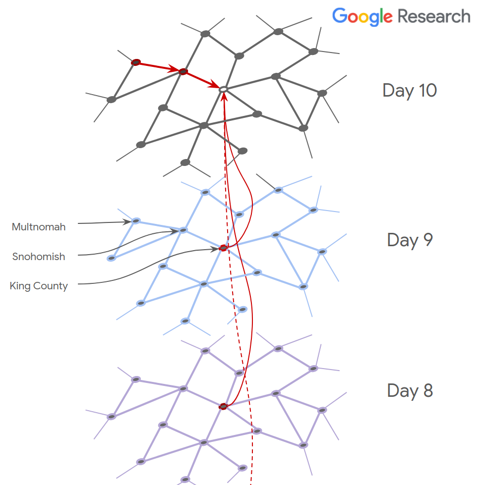
Our own researchers have also explored using this anonymized data to forecast COVID-19 spread using graph neural networks instead of traditional time series-based models.
Although the research community knew little about this disease and secondary effects initially, we’re learning more every day. Our COVID-19 Search Trends symptoms allows researchers to explore temporal or symptomatic associations, such as anosmia — the loss of smell that is sometimes a symptom of the virus. To further support the broader research community, we launched Google Health Studies app to provide the public ways to participate in research studies.
 |
| Our COVID-19 Search Trends are helping researchers study the link between the disease’s spread and symptom-related searches. |
Teams across Google are contributing tools and resources to the broader scientific community, which is working to address the health and economic impacts of the virus.
Accurate information is critical in dealing with public health threats. We collaborated with many product teams at Google in order to improve information quality about COVID-19 in Google News and Search through supporting fact checking efforts, as well as similar efforts in YouTube.
We helped multilingual communities get equal access to critical COVID-19 information by sponsoring localization of Nextstrain.org’s weekly Situation Reports and developing a COVID-19 open source parallel dataset in collaboration with Translators Without Borders.
Modelling a complex global event is particularly challenging and requires more comprehensive epidemiological datasets, the development of novel interpretable models and agent-based simulators to inform the public health response. Machine learning techniques have also helped in other ways from deploying natural language understanding to helping researchers quickly navigate the mountains of COVID-19 scientific literature, applying anonymization technology to protect privacy while making useful datasets available, and exploring whether public health can conduct faster screening with fewer tests via Bayesian group testing.
These are only a sample of the many pieces of work that happened across Google to help users and public health authorities respond to COVID-19. For more, see using technology to help take on COVID-19.
Research in Machine Learning for Medical Diagnostics
We continue to make headway helping clinicians harness the power of ML to deliver better care for more patients. This year we have described notable advances in applying computer vision to aid doctors in the diagnosis and management of cancer, including helping to make sure that doctors don’t miss potentially cancerous polyps during colonoscopies, and showing that an ML system can achieve substantially higher accuracy than pathologists in Gleason grading of prostate tissue, enabling radiologists to achieve significant reductions in both false negative and false positive results when examining X-rays for signs of breast cancer.
 |
| To determine the aggressiveness of prostate cancers, pathologists examine a biopsy and assign it a Gleason grade. In published research, our system was able to grade with higher accuracy than a cohort of pathologists who have not had specialist training in prostate cancer. The first stage of the deep learning system assigns a Gleason grade to every region in a biopsy. In this biopsy, green indicates Gleason pattern 3, while yellow indicates Gleason pattern 4. |
We’ve also been working on systems to help identify skin disease, help detect age-related macular degeneration (the leading cause of blindness in the U.S. and U.K., and the third-largest cause of blindness worldwide), and on potential novel non-invasive diagnostics (e.g., being able to detect signs of anemia from retinal images).
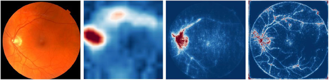 |
| Our study examines how a deep learning model can quantify hemoglobin levels — a measure doctors use to detect anemia — from retinal images. |
This year has also brought exciting demonstrations of how these same technologies can peer into the human genome. Google’s open-source tool, DeepVariant, identifies genomic variants in sequencing data using a convolutional neural network, and this year won the FDA Challenge for best accuracy in 3 out of 4 categories. Using this same tool, a study led by the Dana-Farber Cancer Institute improved diagnostic yield by 14% for genetic variants that lead to prostate cancer and melanoma in a cohort of 2,367 cancer patients.
Research doesn’t end at measurement of experimental accuracy. Ultimately, truly helping patients receive better care requires understanding how ML tools will affect people in the real world. This year we began work with Mayo Clinic to develop a machine learning system to assist in radiotherapy planning and to better understand how this technology could be deployed into clinical practice. With our partners in Thailand, we’ve used diabetic eye disease screening as a test case in how we can build systems with people at the center, and recognize the fundamental role of diversity, equity, and inclusion in building tools for a healthier world.
Weather, Environment and Climate Change
Machine learning can help us better understand the environment and make useful predictions to help people in both their everyday life as well as in disaster situations. For weather and precipitation forecasting, computationally intensive physics-based models like NOAA’s HRRR have long reigned supreme. We have been able to show, though, that ML-based forecasting systems can predict current precipitation with much better spatial resolution (“Is it raining in my local park in Seattle?” and not just “Is it raining in Seattle?”) and can produce short-term forecasts of up to eight hours that are considerably more accurate than HRRR, and can compute the forecast more quickly, yet with higher temporal and spatial resolution.
 |
| A visualization of predictions made over the course of roughly one day. Left: The 1-hour HRRR prediction made at the top of each hour, the limit to how often HRRR provides predictions. Center: The ground truth, i.e., what we are trying to predict. Right: The predictions made by our model. Our predictions are every 2 minutes (displayed here every 15 minutes) at roughly 10 times the spatial resolution made by HRRR. Notice that we capture the general motion and general shape of the storm. |
We’ve also developed an improved technique called HydroNets, which uses a network of neural networks to model the actual river systems in the world to more accurately understand the interactions of upstream water levels to downstream inundation, resulting in more accurate water-level predictions and flood forecasting. Using these techniques, we’ve expanded our coverage of flood alerts by 20x in India and Bangladesh, helping to better protect more than 200 million people in 250,000 square kilometers.
 |
| An illustration of the HydroNets architecture. |
Better analysis of satellite imagery data can also give Google users a better understanding of the impact and extent of wildfires (which caused devastating effects in California and Australia this year). We showed that automated analysis of satellite imagery can help with rapid assessment of damage after natural disasters even with limited prior satellite imagery. It can also aid urban tree-planting efforts by helping cities assess their current tree canopy coverage and where they should focus on planting new trees. We’ve also shown how machine learning techniques that leverage temporal context can help improve ecological and wildlife monitoring.
Based on this work, we’re excited to partner with NOAA on using AI and ML to amplify NOAA’s environmental monitoring, weather forecasting and climate research using Google Cloud’s infrastructure.
Accessibility
Machine learning continues to provide amazing opportunities for improving accessibility, because it can learn to transfer one kind of sensory input into others. As one example, we released Lookout, an Android application that can help visually impaired users by identifying packaged foods, both in a grocery store and also in their kitchen cupboard at home. The machine learning system behind Lookout demonstrates that a powerful-but-compact machine learning model can accomplish this in real-time on a phone for nearly 2 million products.
Similarly, people who communicate with sign language find it difficult to use video conferencing systems because even if they are signing, they are not detected as actively speaking by audio-based speaker detection systems. Developing Real-Time, Automatic Sign Language Detection for Video Conferencing presents a real-time sign language detection model and demonstrates how it can be used to provide video conferencing systems with a mechanism to identify the person signing as the active speaker.
We also enabled useful Android accessibility capabilities such as Voice Access and Sound Notifications for important household sounds.
Live Caption was expanded to support calls on the Pixel phone with the ability to caption phone calls and video calls. This came out of the Live Relay research project, which enables deaf and hard of hearing people to make calls without assistance.
Applications of ML to Other Fields
Machine learning continues to prove vital in helping us make progress across many fields of science. In 2020, in collaboration with the FlyEM team at HHMI Janelia Research Campus, we released the drosophila hemibrain connectome, the large synapse-resolution map of brain connectivity, reconstructed using large-scale machine learning models applied to high-resolution electron microscope imaging of brain tissue. This connectome information will aid neuroscientists in a wide variety of inquiries, helping us all better understand how brains function. Be sure to check out the very fly interactive 3-D UI!
The application of ML to problems in systems biology is also on the rise. Our Google Accelerated Science team, in collaboration with our colleagues at Calico, have been applying machine learning to yeast, to get a better understanding of how genes work together as a whole system. We’ve also been exploring how to use model-based reinforcement learning in order to design biological sequences like DNA or proteins that have desirable properties for medical or industrial uses. Model-based RL is used to improve sample efficiency. At each round of experimentation the policy is trained offline using a simulator fit on functional measurements from prior rounds. On various tasks like designing DNA transcription factor binding sites, designing antimicrobial proteins, and optimizing the energy of Ising models based on protein structures, we find that model-based RL is an attractive alternative to existing methods.
In partnership with X-Chem Pharmaceuticals and ZebiAI, we have also been developing ML techniques to do “virtual screening” of promising molecular compounds computationally. Previous work in this area has tended to focus on relatively small sets of related compounds, but in this work, we are trying to use DNA-encoded small molecule libraries in order to be able to generalize to find “hits” across a wide swath of chemical space, reducing the need for slower, physical-based lab work in order to progress from idea to working pharmaceutical.
We’ve also seen success applying machine learning to core computer science and computer systems problems, a growing trend that is spawning entire new conferences like MLSys. In Learning-based Memory Allocation for C++ Server Workloads, a neural network-based language model predicts context-sensitive per-allocation site object lifetime information, and then uses this to organize the heap so as to reduce fragmentation. It is able to reduce fragmentation by up to 78% while only using huge pages (which are better for TLB behavior). End-to-End, Transferable Deep RL for Graph Optimization described an end-to-end transferable deep reinforcement learning method for computational graph optimization that shows 33%-60% speedup on three graph optimization tasks compared to TensorFlow default optimization, with 15x faster convergence over prior computation graph optimization methods.
 |
| Overview of GO: An end-to-end graph policy network that combines graph embedding and sequential attention. |
As described in Chip Design with Deep Reinforcement Learning, we have also been applying reinforcement learning to the problem of place-and-route in computer chip design. This is normally a very time-consuming, labor-intensive process, and is a major reason that going from an idea for a chip to actually having a fully designed and fabricated chip takes so long. Unlike prior methods, our approach has the ability to learn from past experience and improve over time. In particular, as we train over a greater number of chip blocks, our method becomes better at rapidly generating optimized placements for previously unseen chip blocks. The system is able to generate placements that usually outperform those of human chip design experts, and we have been using this system (running on TPUs) to do placement and layout for major portions of future generations of TPUs. Menger is a recent infrastructure we’ve built for large-scale distributed reinforcement learning that is yielding promising performance for difficult RL tasks such as chip design.
 |
| Macro placements of Ariane, an open-source RISC-V processor, as training progresses. On the left, the policy is being trained from scratch, and on the right, a pre-trained policy is being fine-tuned for this chip. Each rectangle represents an individual macro placement. Notice how the cavity that is occupied by non-macro logic cells that is discovered by the from-scratch policy is already present from the outset in the pre-trained policy’s placement. |
Responsible AI
The Google AI Principles guide our development of advanced technologies. We continue to invest in responsible AI research and tools, update our recommended technical practices in this area, and share regular updates — including a 2020 blog post and report — on our progress in implementation.
To help better understand the behavior of language models, we developed the Language Interpretability Tool (LIT), a toolkit for better interpretability of language models, enabling interactive exploration and analysis of their decisions. We developed techniques for measuring gendered correlations in pre-trained language models and scalable techniques for reducing gender bias in Google Translate. We used the kernel trick to propose a simple method to estimate the influence of a training data example on an individual prediction. To help non-specialists interpret machine learning results, we extended the TCAV technique introduced in 2019 to now provide a complete and sufficient set of concepts. With the original TCAV work, we were able to say that ‘fur’ and ‘long ears’ are important concepts for ‘rabbit’ prediction. With this work, we can also say that these two concepts are enough to fully explain the prediction; you don’t need any other concepts. Concept bottleneck models are a technique to make models more interpretable by training them so that one of the layers is aligned with pre-defined expert concepts (e.g., “bone spurs present”, or “wing color”, as shown below) before making a final prediction for a task, so that we can not only interpret but also turn on/off these concepts on the fly.
In collaboration with many other institutions, we also looked into memorization effects of language models, showing that training data extraction attacks are realistic threats on state-of-the-art large language models. This finding along with a result that embedding models can leak information can have significant privacy implications (especially for models trained on private data). In Thieves of Sesame Street: Model Extraction on BERT-based APIs, we demonstrated that attackers with only API access to a language model could create models whose outputs had very high correlation with the original model, even with relatively few API queries to the original model. Subsequent work demonstrated that attackers can extract smaller models with arbitrary accuracy. On the AI Principle of safety we demonstrated that thirteen published defenses to adversarial examples can be circumvented despite attempting to perform evaluations using adaptive attacks. Our work focuses on laying out the methodology and the approach necessary to perform an adaptive attack, and thus will allow the community to make further progress in building more robust models.
Examining the way in which machine learning systems themselves are examined is also an important area of exploration. In collaboration with the Partnership on AI, we defined a framework for how to audit the use of machine learning in software product settings, drawing on lessons from the aerospace, medical devices, and finance industries and their best practices. In joint work with University of Toronto and MIT, we identified several ethical concerns that can arise when auditing the performance of facial recognition systems. In joint work with the University of Washington, we identified some important considerations related to diversity and inclusion when choosing subsets for evaluating algorithmic fairness. As an initial step in making responsible AI work for the next billion users and to help understand if notions of fairness were consistent in different parts of the world, we analyzed and created a framework for algorithmic fairness in India, accounting for datasets, fairness optimizations, infrastructures, and ecosystems
The Model Cards work that was introduced in collaboration with the University of Toronto in 2019 has been growing in influence. Indeed, many well-known models like OpenAI’s GPT-2 and GPT-3, many of Google’s MediaPipe models and various Google Cloud APIs have all adopted Model Cards as a way of giving users of a machine learning model more information about the model’s development and the observed behavior of the model under different conditions. To make this easier for others to adopt for their own machine learning models, we also introduced the Model Card Toolkit for easier model transparency reporting. In order to increase transparency in ML development practices, we demonstrate the applicability of a range of best practices throughout the dataset development lifecycle, including data requirements specification and data acceptance testing.
In collaboration with the U.S. National Science Foundation (NSF), we announced and helped to fund a National AI Research Institute for Human-AI Interaction and Collaboration. We also released the MinDiff framework, a new regularization technique available in the TF Model Remediation library for effectively and efficiently mitigating unfair biases when training ML models, along with ML-fairness gym for building simple simulations that explore potential long-run impacts of deploying machine learning-based decision systems in social environments.
In addition to developing frameworks for fairness, we developed approaches for identifying and improving the health and quality of experiences with Recommender Systems, including using reinforcement learning to introduce safer trajectories. We also continue to work on improving the reliability of our machine learning systems, where we’ve seen that approaches such as generating adversarial examples can improve robustness and that robustness approaches can improve fairness.
Differential privacy is a way to formally quantify privacy protections and requires a rethinking of the most basic algorithms to operate in a way that they do not leak information about any particular individual. In particular, differential privacy can help in addressing memorization effects and information leakage of the kinds mentioned above. In 2020 there were a number of exciting developments, from more efficient ways of computing private empirical risk minimizers to private clustering methods with tight approximation guarantees and private sketching algorithms. We also open sourced the differential privacy libraries that lie at the core of our internal tools, taking extra care to protect against leakage caused by the floating point representation of real numbers. These are the exact same tools that we use to produce differentially private COVID-19 mobility reports that have been a valuable source of anonymous data for researchers and policymakers.
To help developers assess the privacy properties of their classification models we released an ML privacy testing library in Tensorflow. We hope this library will be the starting point of a robust privacy testing suite that can be used by any machine learning developer around the world.
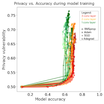 |
| Membership inference attack on models for CIFAR10. The x-axis is the test accuracy of the model, and y-axis is vulnerability score (lower means more private). Vulnerability grows while test accuracy remains the same — better generalization could prevent privacy leakage. |
In addition to pushing the state of the art in developing private algorithms, I am excited about the advances we made in weaving privacy into the fabric of our products. One of the best examples is Chrome’s Privacy Sandbox, which changes the underpinnings of the advertising ecosystem and helps systematically protect individuals’ privacy. As part of the project, we proposed and evaluated a number of different APIs, including federated learning of cohorts (FLoC) for interest based targeting, and aggregate APIs for differentially private measurement.
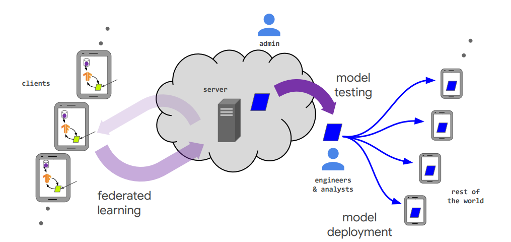
Launched in 2017, federated learning is now a complete research field unto itself, with over 3000 publications on federated learning appearing in 2020 alone. Our cross-institutional Advances and Open Problems in Federated Learning survey paper published in 2019 has been cited 367 times in the past year, and an updated version will soon be published in the Foundations & Trends in Machine Learning series. In July, we hosted a Workshop on Federated Learning and Analytics, and made all research talks and a TensorFlow Federated tutorial publicly available.
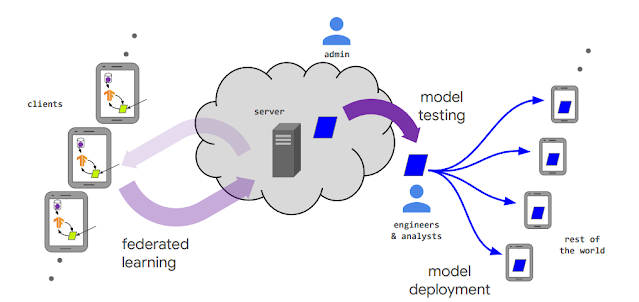 |
| The lifecycle of an FL-trained model and the various actors in a federated learning system. |
We continue to push the state of the art in federated learning, including the development of new federated optimization algorithms including adaptive learning algorithms, posterior averaging algorithms, and techniques for mimicking centralized algorithms in federated settings, substantial improvements in complimentary cryptographic protocols, and more. We announced and deployed federated analytics, enabling data science over raw data that is stored locally on users’ devices. New uses of federated learning in Google products include contextual emoji suggestions in Gboard, and pioneering privacy-preserving medical research with Google Health Studies. Furthermore, in Privacy Amplification via Random Check-Ins we presented the first privacy accounting mechanism for Federated Learning.
Security for our users is also an area of considerable interest for us. In 2020, we continued to improve protections for Gmail users, by deploying a new ML-based document scanner that provides protection against malicious documents, which increased malicious office document detection by 10% on a daily basis. Thanks to its ability to generalize, this tool has been very effective at blocking some adversarial malware campaigns that elude other detection mechanisms and increased our detection rate by 150% in some cases.
On the account protection side, we released a fully open-source security key firmware to help advance state of art in the two factor authentication space, staying focused on security keys as the best way to protect accounts against phishing.
Natural Language Understanding
Better understanding of language is an area where we saw considerable progress this year. Much of the work in this space from Google and elsewhere now relies on Transformers, a particular style of neural network model originally developed for language problems (but with a growing body of evidence that they are also useful for images, videos, speech, protein folding, and a wide variety of other domains).
One area of excitement is in dialog systems that can chat with a user about something of interest, often encompassing multiple turns of interaction. While successful work in this area to date has involved creating systems that are specialized around particular topics (e.g., Duplex) these systems cannot carry on general conversations. In pursuit of the general research goal of creating systems capable of much more open-ended dialog, in 2020 we described Meena, a learned conversational agent that aspirationally can chat about anything. Meena achieves high scores on a dialog system metric called SSA, which measures both sensibility and specificity of responses. We’ve seen that as we scale up the model size of Meena, it is able to achieve lower perplexity and, as shown in the paper, lower perplexity correlates extremely closely with improved SSA.
 |
| A chat between Meena (left) and a person (right). |
One well-known issue with generative language models and dialog systems is that when discussing factual data, the model’s capacity may not be large enough to remember every specific detail about a topic, so they generate language that is plausible but incorrect. (This is not unique to machines — people can commit these errors too.) To address this in dialog systems, we are exploring ways to augment a conversational agent by giving it access to external information sources (e.g., a large corpus of documents or a search engine API), and developing learning techniques to use this as an additional resource in order to generate language that is consistent with the retrieved text. Work in this area includes integrating retrieval into language representation models (and a key underlying technology for this to work well is something like ScaNN, an efficient vector similarity search, to efficiently match the desired information to information in the corpus of text). Once appropriate content is found, it can be better understood with approaches like using neural networks to find answers in tables and extracting structured data from templatic documents. Our work on PEGASUS, a state-of-the-art model for abstractive text summarization can also help to create automatic summaries from any piece of text, a general technique useful in conversations, retrieval systems, and many other places.
Efficiency of NLP models has also been a significant focus for our work in 2020. Techniques like transfer learning and multi-task learning can dramatically help with making general NLP models usable for new tasks with modest amounts of computation. Work in this vein includes transfer learning explorations in T5, sparse activation of models (as in our GShard work mentioned below), and more efficient model pre-training with ELECTRA. Several threads of work also look to improve on the basic Transformer architecture, including Reformer, which uses locality-sensitive hashing and reversible computation to more efficiently support much larger attention windows, Performers, which use an approach for attention that scales linearly rather than quadratically (and discusses its use in the context of protein modeling), and ETC and BigBird, which utilize global and sparse random connections, to enable linear scaling for larger and structured sequences. We also explored techniques for creating very lightweight NLP models that are 100x smaller than a larger BERT model, but perform nearly as well for some tasks, making them very suitable for on-device NLP. In Encode, Tag and Realize, we also explored new approaches for generative text models that use edit operations rather than fully general text generation, which can have advantages in computation requirements for generation, more control over the generated text, and require less training data.
Language Translation
Effective language translation helps bring the world closer together by enabling us to all communicate, despite speaking different languages. To date, over a billion people around the world use Google Translate, and last year we added support for five new languages (Kinyarwanda, Odia, Tatar, Turkmen and Uyghur, collectively spoken by 75 million people). Translation quality continues to improve, showing an average +5 BLEU point gain across more than 100 languages from May 2019 to May 2020, through a wide variety of techniques like improved model architectures and training, better handling of noise in datasets, multilingual transfer and multi-task learning, and better use of monolingual data to improve low-resource languages (those without much written public content on the web), directly in line with our goals of improving ML fairness of machine learning systems to provide benefits to the greatest number of people possible.
We strongly believe that continued scaling of multilingual translation models will bring further quality improvements, especially to the billions of speakers of low-resource languages around the world. In GShard: Scaling Giant Models with Conditional Computation and Automatic Sharding, Google researchers showed that training sparsely-activated multilingual translation models of up to 600 billion parameters leads to major improvements in translation quality for 100 languages as measured by BLEU score improvement over a baseline of a separate 400M parameter monolingual baseline model for each language. Three trends stood out in this work, illustrated by Figure 6 in the paper, reproduced below (see the paper for complete discussion):
- The BLEU score improvements from multilingual training are high for all languages but are even higher for low-resource languages (right hand side of graph is higher than the left) whose speakers represent billions of people in some of the world’s most marginalized communities. Each rectangle on the figure represents languages with 1B speakers.
- The larger and deeper the model, the larger the BLEU score improvements were across all languages (the lines hardly ever cross).
- Large, sparse models also show a ~10x to 100x improvement in computational efficiency for model training over training a large, dense model, while simultaneously matching or significantly exceeding the BLEU scores of the large, dense model (computational efficiency discussed in paper).
We’re actively working on bringing the benefits demonstrated in this GShard research work to Google Translate, as well as training single models that cover 1000 languages, including languages like Dhivehi and Sudanese Arabic (while sharing some challenges that needed solving along the way).
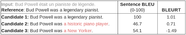
We also developed techniques to create language-agnostic representations of sentences for BERT models, which can help with developing better translation models. To more effectively evaluate translation quality, we introduced BLEURT, a new metric for evaluating language generation for tasks like translation that considers the semantics of the generated text, rather than just the amount of word overlap with ground-truth data, illustrated in the table below.
Machine Learning Algorithms
We continue to develop new machine learning algorithms and approaches for training that enable systems to learn more quickly and from less supervised data. By replaying intermediate results during training of neural networks, we find that we can fill idle time on ML accelerators and therefore can train neural networks faster. By changing the connectivity of neurons dynamically during training, we can find better solutions compared with statically-connected neural networks. We also developed SimCLR, a new self-supervised and semi-supervised learning technique that simultaneously maximizes agreement between differently transformed views of the same image and minimizes agreement between transformed views of different images. This approach significantly improves on the best self-supervised learning techniques.
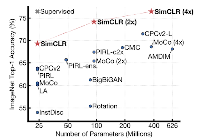 |
| ImageNet top-1 accuracy of linear classifiers trained on representations learned with different self-supervised methods (pretrained on ImageNet). Gray cross indicates supervised ResNet-50. |
We also extended the idea of contrastive learning to the supervised regime, resulting in a loss function that significantly improves over cross-entropy for supervised classification problems.
Reinforcement Learning
Reinforcement learning (RL), which learns to make good long-term decisions from limited experience, has been an important focus area for us. An important challenge in RL is to learn to make decisions from few data points, and we’ve improved RL algorithm efficiency through learning from fixed datasets, learning from other agents, and improving exploration.
A major focus area this year has been around offline RL, which relies solely on fixed, previously collected datasets (for example, from previous experiments or human demonstrations), extending RL to the applications that can’t collect training data on-the-fly. We’ve introduced a duality approach to RL, developed improved algorithms for off-policy evaluation, estimating confidence intervals, and offline policy optimization. In addition, we’re collaborating with the broader community to tackle these problems by releasing open-source benchmark datasets, and DQN dataset for Atari.
 |
| Offline RL on Atari games using the DQN Replay Dataset. |
Another line of research improved sample efficiency by learning from other agents through apprenticeship learning. We developed methods to learn from informed agents, matching other agent’s distribution, or learning from adversarial examples. To improve the exploration in RL, we explored bonus-based exploration methods including imitation techniques able to mimic structured exploration arising in agents having prior knowledge about their environment.
We’ve also made significant advances in the mathematical theory of reinforcement learning. One of our main areas of research was studying reinforcement learning as an optimization process. We found connections to the Frank-Wolfe algorithm, momentum methods, KL divergence regularization, operator theory, and convergence analysis; some of these insights led to an algorithm that achieves state-of-the-art performance in challenging RL benchmarks and discovery that polynomial transfer functions avoid convergence problems associated with softmax, both in RL and supervised learning. We’ve made some exciting progress on the topic of safe reinforcement learning, where one seeks to discover optimal control rules while respecting important experimental constraints. This includes a framework for safe policy optimization. We studied efficient RL-based algorithms for solving a class of problems known as mean field games, which model systems with a large number of decision-makers, from mobile networks to electric grids.
We’ve made breakthroughs toward generalization to new tasks and environments, an important challenge for scaling up RL to complex real-world problems. A 2020 focus area was population-based learning-to-learn methods, where another RL or evolutionary agent trained a population of RL agents to create a curriculum of emergent complexity, and discover new state-of-the-art RL algorithms. Learning to estimate the importance of data points in the training set and parts of visual input with selective attention resulted in significantly more skillful RL agents.
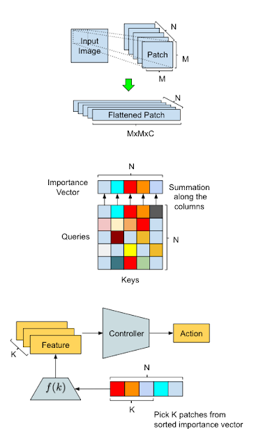 |
| Overview of our method and illustration of data processing flow in AttentionAgent. Top: Input transformation — A sliding window segments an input image into smaller patches, and then “flattens” them for future processing. Middle: Patch election — The modified self-attention module holds votes between patches to generate a patch importance vector. Bottom: Action generation — AttentionAgent picks the patches of the highest importance, extracts corresponding features and makes decisions based on them. |
Further, we made progress in model-based RL by showing that learning predictive behavior models accelerates RL learning, and enables decentralized cooperative multi-agent tasks in diverse teams, and learning long-term behavior models. Observing that skills bring predictable changes in the environment, we discover skills without supervision. Better representations stabilize RL learning, while hierarchical latent spaces and value-improvement paths yield better performance.
We shared open source tools for scaling up and productionizing RL. To expand the scope and problems tackled by users, we’ve introduced SEED, a massively parallel RL agent, released a library for measuring the RL algorithm reliability, and a new version of TF-Agents that includes distributed RL, TPU support, and a full set of bandit algorithms. In addition, we performed a large empirical study of RL algorithms to improve hyperparameter selection and algorithm design.
Finally, in collaboration with Loon, we trained and deployed RL to more efficiently control stratospheric balloons, improving both power usage and their ability to navigate.
AutoML
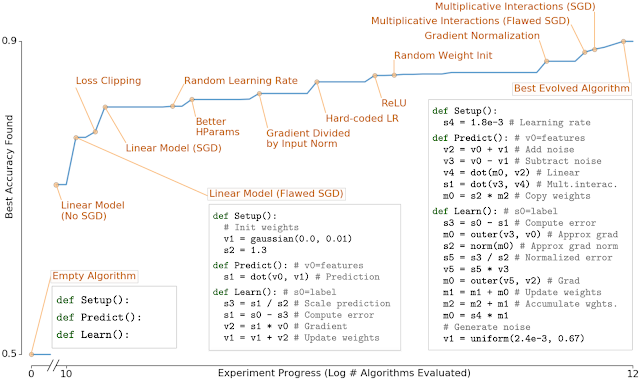
Using learning algorithms to develop new machine learning techniques and solutions, or meta-learning, is a very active and exciting area of research. In much of our previous work in this area, we’ve created search spaces that look at how to find ways to combine sophisticated hand-designed components together in interesting ways. In AutoML-Zero: Evolving Code that Learns, we took a different approach, by giving an evolutionary algorithm a search space consisting of very primitive operations (like addition, subtraction, variable assignment, and matrix multiplication) in order to see if it was possible to evolve modern ML algorithms from scratch. The presence of useful learning algorithms in this space is incredibly sparse, so it is remarkable that the system was able to progressively evolve more and more sophisticated ML algorithms. As shown in the figure below, the system reinvents many of the most important ML discoveries over the past 30 years, such as linear models, gradient descent, rectified linear units, effective learning rate settings and weight initializations, and gradient normalization.
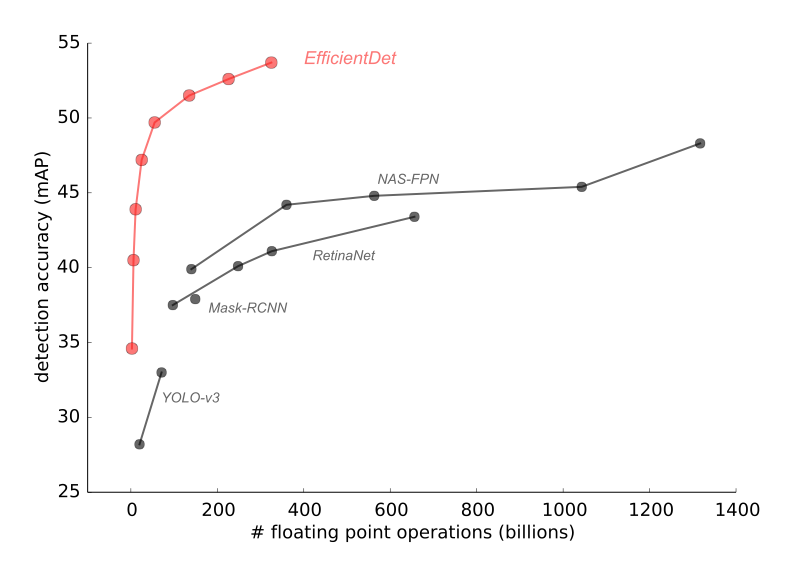
We also used meta-learning to discover a variety of new efficient architectures for object detection in both still images and videos. Last year’s work on EfficientNet for efficient image classification architectures showed significant accuracy improvements and computational cost reductions for image classification. In follow-on work this year, EfficientDet: Towards Scalable and Efficient Object Detection builds on top of the EfficientNet work to derive new efficient architectures for object detection and localization, showing remarkable improvements in both highest absolute accuracy, as well as computational cost reductions of 13-42x over previous approaches to achieve a given level of accuracy.
 |
| EfficientDet achieves state-of-the-art 52.2 mAP, up 1.5 points from the prior state of the art (not shown since it is at 3045B FLOPs) on COCO test-dev under the same setting. Under the same accuracy constraint, EfficientDet models are 4x-9x smaller and use 13x-42x less computation than previous detectors. |
Our work on SpineNet describes a meta-learned architecture that can retain spatial information more effectively, allowing detection to be done at finer resolution. We also focused on learning effective architectures for a variety of video classification problems. AssembleNet: Searching for Multi-Stream Neural Connectivity in Video Architectures, AssembleNet++: Assembling Modality Representations via Attention Connections, and AttentionNAS: Spatiotemporal Attention Cell Search for Video Classification demonstrate how to use evolutionary algorithms to create novel state-of-the-art video processing machine learning architectures.
This approach can also be used to develop effective model architectures for time series forecasting. Using AutoML for Time Series Forecasting describes the system that discovers new forecasting models via an automated search over a search space involving many interesting kinds of low-level building blocks, and its effectiveness was demonstrated in the Kaggle M5 Forecasting Competition, by generating an algorithm and system that placed 138th out of 5558 participants (top 2.5%). While many of the competitive forecasting models required months of manual effort to create, our AutoML solution found the model in a short time with only a moderate compute cost (500 CPUs for 2 hours) and no human intervention.
Better Understanding of ML Algorithms and Models
Deeper understanding of machine learning algorithms and models is crucial for designing and training more effective models, as well as understanding when models may fail. Last year, we focused on fundamental questions around representation power, optimization, model generalization, and label noise, among others. As mentioned earlier in this post, Transformer networks have had a huge impact on modeling language, speech and vision problems, but what is the class of functions represented by these models? Recently we showed that transformers are universal approximators for sequence-to-sequence functions. Furthermore, sparse transformers also remain universal approximators even when they use just a linear number of interactions among the tokens. We have been developing new optimization techniques based on layerwise adaptive learning rates to improve the convergence speed of transformers, e.g., Large batch optimization for deep learning (LAMB): Training BERT in 76 minutes.
As neural networks are made wider and deeper, they often train faster and generalize better. This is a core mystery in deep learning since classical learning theory suggests that large networks should overfit more. We are working to understand neural networks in this overparameterized regime. In the limit of infinite width, neural networks take on a surprisingly simple form, and are described by a Neural Network Gaussian Process (NNGP) or Neural Tangent Kernel (NTK). We studied this phenomenon theoretically and experimentally, and released Neural Tangents, an open-source software library written in JAX that allows researchers to build and train infinite-width neural networks.
 |
| Left: A schematic showing how deep neural networks induce simple input / output maps as they become infinitely wide. Right: As the width of a neural network increases, we see that the distribution of outputs over different random instantiations of the network becomes Gaussian. |
As finite width networks are made larger, they also demonstrate peculiar double descent phenomena — where they generalize better, then worse, then better again with increasing width. We have shown that this phenomenon can be explained by a novel bias-variance decomposition, and further that it can sometimes manifest as triple descent.
Lastly, in real-world problems, one often needs to deal with significant label noise. For instance, in large scale learning scenarios, weakly labeled data is available in abundance with large label noise. We have developed new techniques for distilling effective supervision from severe label noise leading to state-of-the-art results. We have further analyzed the effects of training neural networks with random labels, and shown that it leads to alignment between network parameters and input data, enabling faster downstream training than initializing from scratch. We have also explored questions such as whether label smoothing or gradient clipping can mitigate label noise, leading to new insights for developing robust training techniques with noisy labels.
Algorithmic Foundations and Theory
2020 was a productive year for our work in algorithmic foundations and theory, with several impactful research publications and notable results. On the optimization front, our paper on edge-weighted online bipartite matching develops a new technique for online competitive algorithms and solves a thirty-year old open problem for the edge-weighted variant with applications in efficient online ad allocation. Along with this work in online allocation, we developed dual mirror descent techniques that generalize to a variety of models with additional diversity and fairness constraints, and published a sequence of papers on the topic of online optimization with ML advice in online scheduling, online learning and online linear optimization. Another research result gave the first improvement in 50 years on the classic bipartite matching in dense graphs. Finally, another paper solves a long-standing open problem about chasing convex bodies online — using an algorithm from The Book, no less.
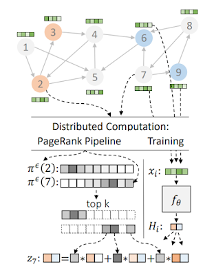
We also continued our work in scalable graph mining and graph-based learning and hosted the Graph Mining & Learning at Scale Workshop at NeurIPS’20, which covered work on scalable graph algorithms including graph clustering, graph embedding, causal inference, and graph neural networks. As part of the workshop, we showed how to solve several fundamental graph problems faster, both in theory and practice, by augmenting standard synchronous computation frameworks like MapReduce with a distributed hash-table similar to a BigTable. Our extensive empirical study validates the practical relevance of the AMPC model inspired by our use of distributed hash tables in massive parallel algorithms for hierarchical clustering and connected components, and our theoretical results show how to solve many of these problems in constant distributed rounds, greatly improving upon our previous results. We also achieved exponential speedup for computing PageRank and random walks. On the graph-based learning side, we presented Grale, our framework for designing graphs for use in machine learning. Furthermore, we presented our work on more scalable graph neural network models, where we show that PageRank can be used to greatly accelerate inference in GNNs.
In market algorithms, an area at the intersection of computer science and economics, we continued our research in designing improved online marketplaces, such as measuring incentive properties of ad auctions, two-sided markets, and optimizing order statistics in ad selection. In the area of repeated auctions, we developed frameworks to make dynamic mechanisms robust against lack of forecasting or estimation errors of the current market and/or the future market, leading to provably tight low-regret dynamic mechanisms. Later, we characterized when it is possible to achieve the asymptotically optimal objective through geometry-based criteria. We also compared the equilibrium outcome of a range of budget management strategies used in practice, showed their impact on the tradeoff between revenue and buyers’ utility and shed light on their incentive properties. Additionally, we continued our research in learning optimal auction parameters, and settled the complexity of batch-learning with revenue loss. We designed the optimal regret and studied combinatorial optimization for contextual auction pricing, and developed a new active learning framework for auctions and improved the approximation for posted-price auctions. Finally, motivated by the importance of incentives in ad auctions, and in the hope to help advertisers study the impact of incentives in auctions, we introduce a data-driven metric to quantify how much a mechanism deviates from incentive compatibility.
Machine Perception
Perceiving the world around us — understanding, modeling and acting on visual, auditory and multimodal input — continues to be a research area with tremendous potential to be beneficial in our everyday lives.
In 2020, deep learning powered new approaches that bring 3D computer vision and computer graphics closer together. CvxNet, deep implicit functions for 3D shapes, neural voxel rendering and CoReNet are a few examples of this direction. Furthermore, our research on representing scenes as neural radiance fields (aka NeRF, see also this blog post) is a good example of how Google Research’s academic collaborations stimulate rapid progress in the area of neural volume rendering.
In Learning to Factorize and Relight a City, a collaboration with UC Berkeley, we proposed a learning-based framework for disentangling outdoor scenes into temporally-varying illumination and permanent scene factors. This gives the ability to change lighting effects and scene geometry for any Street View panorama, or even turn it into a full-day timelapse video.
Our work on generative human shape and articulated pose models introduces a statistical, articulated 3D human shape modeling pipeline, within a fully trainable, modular, deep learning framework. Such models enable 3D human pose and shape reconstruction of people from a single photo to better understand the scene.
The growing area of media compression using neural networks continued to make strong progress in 2020, not only on learned image compression, but also in deep approaches to video compression, volume compression and nice results in deep distortion-agnostic image watermarking.
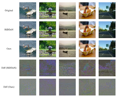 |
| Samples of encoded and cover images for Distortion Agnostic Deep Watermarking. First row: Cover image with no embedded message. Second row: Encoded image from HiDDeN combined distortion model. Third row: Encoded images from our model. Fourth row: Normalized difference of the encoded image and cover image for the HiDDeN combined model. Fifth row: Normalized difference for our model |
Additional important themes in perceptual research included:
- Making better use of data (e.g., self-training with noisy students, learning from simulated data, learning with noisy labels, contrastive learning)
- Reasoning across modalities (e.g., exploiting cross-modal supervision, audiovisual speech enhancement, language grounding, Open Images (V6) update featuring localized narratives — multimodal annotations connecting vision and language)
- Developing approaches for efficient perception, particularly on edge devices (e.g., fast sparse convnets, structured multi-hashing for model compression)
- Improving the ability to represent and reason about objects and scenes (e.g., detecting 3D objects and predicting 3D shapes, 3D scene reconstruction from a single RGB image, leveraging temporal context for object detection, learning to see transparent objects and estimating their pose from stereo)
- AI enabling human creativity (e.g., automatic creation of videos from web pages, intelligent video reframing, using GANs to create fantastical creatures, relighting portraits)
Engaging with the broader research community through open sourcing of solutions and datasets is another important aspect of furthering perceptual research. In 2020, we open sourced multiple new perceptual inference capabilities and solutions in MediaPipe, such as on-device face, hand and pose prediction, real-time body pose tracking, real-time iris tracking and depth estimation, and real-time 3D object detection.
We continued to make strides to improve experiences and promote helpfulness on mobile devices through ML-based solutions. Our ability to run sophisticated natural language processing on-device, enabling more natural conversational features, continues to improve. In 2020, we expanded Call Screen and launched Hold for Me to allow users to save time when performing mundane tasks, and we also launched language-based actions and language navigability of our Recorder app to aid productivity.
We have used Google’s Duplex technology to make calls to businesses and confirm things like temporary closures. This has enabled us to make 3 million updates to business information globally, that have been seen over 20 billion times on Maps and Search. We also used text to speech technology for easier access to web pages, by enabling Google Assistant to read it aloud, supporting 42 languages.
We also continued to make meaningful improvements to imaging applications. We made it easier to capture precious moments on Pixel with innovative controls and new ways to relight, edit, enhance and relive them again in Google Photos. For the Pixel camera, beginning with Pixel 4 and 4a, we added Live HDR+, which uses machine learning to approximate the vibrance and balanced exposure and appearance of HDR+ burst photography in real time in the viewfinder. We also created dual exposure controls, which allow the brightness of shadows and highlights in a scene to be adjusted independently — live in the viewfinder.
More recently, we introduced Portrait Light, a new post-capture feature for the Pixel Camera and Google Photos apps that adds a simulated directional light source to portraits. This feature is again one that is powered by machine learning, having been trained on 70 different people, photographed one light at a time, in our pretty cool 331-LED Light Stage computational illumination system.
In the past year, Google researchers were excited to contribute to many new (and timely) ways of using Google products. Here are a few examples
Robotics
In the area of robotics research, we’ve made tremendous progress in our ability to learn more and more complex, safe and robust robot behaviors with less and less data, using many of the RL techniques described earlier in the post.
Transporter Networks are a novel approach to learning how to represent robotic tasks as spatial displacements. Representing relations between objects and the robot end-effectors, as opposed to absolute positions in the environment, makes learning robust transformations of the workspace very efficient.
In Grounding Language in Play, we demonstrated how a robot can be taught to follow natural language instructions (in many languages!). This required a scalable approach to collecting paired data of natural language instructions and robot behaviors. One key insight is that this can be accomplished by asking robot operators to simply play with the robot, and label after-the-fact what instructions would have led to the robot accomplishing the same task.
We also explored doing away with robots altogether (by having humans use a camera-equipped grasping stick) for even more scalable data collection, and how to efficiently transfer visual representations across robotic tasks.
We investigated how to learn very agile strategies for robot locomotion, by taking inspiration from nature, using evolutionary meta-learning strategies, human demonstrations, and various approaches to training data-efficient controllers using deep reinforcement learning.
One increased emphasis this year has been on safety: how do we deploy safe delivery drones in the real world? How do we explore the world in a way that always allows the robot to recover from its mistakes? How do we certify the stability of learned behaviors? This is a critical area of research on which we expect to see increased focus in the future.
Quantum Computing
Our Quantum AI team continued its work to establish practical uses of quantum computing. We ran experimental algorithms on our Sycamore processors to simulate systems relevant to chemistry and physics. These simulations are approaching a scale at which they can not be performed on classical computers anymore, making good on Feynman’s original idea of using quantum computers as an efficient means to simulate systems in which quantum effects are important. We published new quantum algorithms, for instance to perform precise processor calibration, to show an advantage for quantum machine learning or to test quantum enhanced optimization. We also worked on programming models to make it easier to express quantum algorithms. We released qsim, an efficient simulation tool to develop and test quantum algorithms with up to 40 qubits on Google Cloud.
We continued to follow our roadmap towards building a universal error-corrected quantum computer. Our next milestone is the demonstration that quantum error correction can work in practice. To achieve this, we will show that a larger grid of qubits can hold logical information exponentially longer than a smaller grid, even though individual components such as qubits, couplers or I/O devices have imperfections. We are also particularly excited that we now have our own cleanroom which should significantly increase the speed and quality of our processor fabrication.
Supporting the Broader Developer and Researcher Community
This year marked TensorFlow’s 5th birthday, passing 160M downloads. The TensorFlow community continued its impressive growth with new special interest groups, TensorFlow User Groups, TensorFlow Certificates, AI Service partners, and inspiring demos #TFCommunitySpotlight. We significantly improved TF 2.x with seamless TPU support, out of the box performance (and best-in-class performance on MLPerf 0.7), data preprocessing, distribution strategy, and a new NumPy API.
We also added many more capabilities to the TensorFlow Ecosystem to help developers and researchers in their workflows: Sounds of India demonstrated going from research to production in under 90 days, using TFX for training and TF.js for deployment in the browser. With Mesh TensorFlow, we pushed the boundaries of model parallelism to provide ultra-high image resolution image analysis. We open-sourced the new TF runtime, TF Profiler for model performance debugging, and tools for Responsible AI, such as the Model Card Toolkit for model transparency and a privacy testing library. With TensorBoard.dev we made it possible to easily host, track, and share your ML experiments for free.
In addition, we redoubled our investment in JAX, an open-source, research-focused ML system that has been actively developed over the past two years. Researchers at Google and beyond are now using JAX in a wide range of fields, including differential privacy, neural rendering, physics-informed networks, fast attention, molecular dynamics, tensor networks, neural tangent kernels, and neural ODEs. JAX accelerates research at DeepMind, powering a growing ecosystem of libraries and work on GANs, meta-gradients, reinforcement learning, and more. We also used JAX and the Flax neural network library to build record-setting MLPerf benchmark submissions, which we demonstrated live at NeurIPS on a large TPU Pod slice with a next-generation Cloud TPU user experience (slides, video, sign-up form). Finally, we’re ensuring that JAX works seamlessly with TF ecosystem tooling, from TF.data for data preprocessing and TensorBoard for experiment visualization to the TF Profiler for performance debugging, with more to come in 2021.
Many recent research breakthroughs have been enabled by increased computing power, and we make more than 500 petaflops of Cloud TPU computing power available for free to researchers around the world via the TFRC program to help broaden access to the machine learning research frontier. More than 120 TFRC-supported papers have been published to date, many of which would not have been possible without the computing resources that the program provides. For example, TFRC researchers have recently developed simulations of wildfire spread, helped analyze COVID-19 content and vaccine sentiment changes on social media networks, and advanced our collective understanding of the lottery ticket hypothesis and neural network pruning. Members of the TFRC community have also published experiments with Persian poetry, won a Kaggle contest on fine-grained fashion image segmentation, and shared tutorials and open-source tools as starting points for others. In 2021, we will change the name of the TFRC program to the TPU Research Cloud program to be more inclusive now that Cloud TPUs support JAX and PyTorch in addition to TensorFlow.
Finally, this was a huge year for Colab. Usage doubled, and we launched productivity features to help people do their work more efficiently, including improved Drive integration and access to the Colab VM via the terminal. And we launched Colab Pro to enable users to access faster GPUs, longer runtimes and more memory.
Open Datasets and Dataset Search
Open datasets with clear and measurable goals are often very helpful in driving forward the field of machine learning. To help the research community find interesting datasets, we continue to index a wide variety of open datasets sourced from many different organizations with Google Dataset Search. We also think it’s important to create new datasets for the community to explore and to develop new techniques, while ensuring that we share open data responsibly. This year, in addition to open datasets to help address the COVID crisis, we released a number of open datasets across many different areas:
- An Analysis of Online Datasets Using Dataset Search (Published, in Part, as a Dataset): a meta dataset about datasets!
- Google Compute Cluster Trace Data: in 2011, Google published a trace of 29 days of compute activity on one of our compute clusters, which has proven very useful for the computer systems community to explore job scheduling policies, better understand utilization in these clusters, etc. This year we published a larger and more extensive version of this data, covering eight of our compute clusters with much finer-grained information.
- Announcing the Objectron Dataset: a collection of 15,000 short, object-centric video clips annotated with 3-D bounding boxes, capturing a larger set of common objects from different angles, as well as 4M annotated images collected from a geo-diverse sample (covering 10 countries across five continents).
- Open Images V6 — Now Featuring Localized Narratives: in addition to the 9M images annotated with 36M image-level labels, 15.8M bounding boxes, 2.8M instance segmentations, and 391k visual relationships found in version 5, this new release adds localized narratives, a completely new form of multimodal annotations that consist of synchronized voice, text, and mouse traces over the objects being described. In Open Images V6, these localized narratives are available for 500k of its images. Additionally, in order to facilitate comparison to previous works, we also release localized narratives annotations for the full 123k images of the COCO dataset.
- A Challenge and Workshop in Efficient Open-Domain Question Answering, created in collaboration with researchers from University of Washington and Princeton, aims to challenge researchers to create systems capable of answering arbitrary questions. A technical report describes the competition and workshop that happened at NeurIPS 2020.
- TyDi QA: A Multilingual Question Answering Benchmark discusses a new benchmark for measuring effectiveness of multilingual question answering (since many benchmarks in this area are English-only or otherwise monolingual, and we feel answering questions in any language is important).
- Wiki-40B: Multilingual Language Model Dataset is a new multilingual language model benchmark that is composed of 40+ languages spanning several scripts and linguistic families. With around 40 billion characters, we hope this new resource will accelerate the research of multilingual modeling. We also released high quality trained language models trained on this dataset, enabling easy comparison of different techniques with these baselines.
- XTREME: A Massively Multilingual Multi-task Benchmark for Evaluating Cross-lingual Generalization can help assess progress on cross-lingual generalizations in a multi-task setting.
- How to Ask Better Questions? A Large-Scale Multi-Domain Dataset for Rewriting Ill-Formed Questions presents a dataset of 427,719 question pairs across 303 domains that can be used to train models to rewrite poorly-formed questions into better formulations.
- Open-Sourcing Big Transfer (BiT): Exploring Large-Scale Pre-training for Computer Vision describes an open-sourced pre-trained model that can be used as a starting point for a wide variety of image-related tasks.
- The 2020 Image Matching Benchmark and Challenge is a dataset and benchmark challenge for the problem of capturing 3D structure from motion (either from videos, or from many images of a scene from many different angles), created in collaboration with University of Victoria, Czech Technical University, and EPFL.
- Meta-Dataset: A Dataset of Datasets for Few-Shot Learning is a dataset of datasets. One of the long-term goals in ML is to build systems that can generalize not from one example to another within the same task, but can generalize even across tasks to solve new problems with little or no training. This meta-dataset can allow us to measure progress towards this ultimate goal.
- Google Landmarks Dataset v2 – A Large-Scale Benchmark for Instance-Level Recognition and Retrieval introduces the Google Landmarks Dataset v2 (GLDv2), a new benchmark for large-scale, fine-grained instance recognition and image retrieval in the domain of human-made and natural landmarks. GLDv2 is the largest such dataset to date by a large margin, including over 5M images and 200k distinct instance labels. Its test set consists of 118k images with ground truth annotations for both the retrieval and recognition tasks.
- Enhancing the Research Community’s Access to Street View Panoramas for Language Grounding Tasks describes a new open dataset to allow researchers to compare techniques for language-grounded navigation tasks or other tasks that rely on Street View panoramas, using a well-known set of data so that comparisons between different techniques can be done more easily.
Research Community Interaction
We are proud to enthusiastically support and participate in the broader research community. In 2020, Google researchers presented over 500 papers at leading research conferences, additionally serving on program committees, organizing workshops, tutorials and numerous other activities aimed at collectively progressing the state of the art in the field. To learn more about our contributions to some of the larger research conferences this year, please see our blog posts for ICLR 2020, CVPR 2020, ACL 2020, ICML 2020, ECCV 2020 and NeurIPS 2020.
In 2020 we supported external research with $37M in funding, including $8.5M in COVID research, $8M in research inclusion and equity, and $2M in responsible AI research. In February, we announced the 2019 Google Faculty Research Award Recipients, funding research proposals from 150 faculty members throughout the world. Among this group, 27% self-identified as members of historically underrepresented groups within technology. We also announced a new Research Scholar Program to support early-career professors who are pursuing research in fields relevant to Google via unrestricted gifts. As we have for more than a decade, we selected a group of incredibly talented PhD student researchers to receive Google PhD Fellowships, which provides funding for graduate studies, as well as mentorship as they pursue their research, and opportunities to interact with other Google PhD Fellows.
We are also expanding the ways that we support inclusion and bring new voices into the field of computer science. In 2020, we created a new Award for Inclusion Research program that supports academic research in computing and technology addressing the needs of underrepresented populations. In the inaugural set of awards, we selected 16 proposals for funding with 25 principal investigators, focused on topics around diversity and inclusion, algorithmic bias, education innovation, health tools, accessibility, gender bias, AI for social good, security, and social justice. We additionally partnered with the Computing Alliance of Hispanic-Serving Institutions (CAHSI) and the CMD-IT Diversifying Future Leadership in the Professoriate Alliance (FLIP) to create an award program for doctoral students from traditionally underrepresented backgrounds to support the last year of the completion of the dissertation requirements.
In 2019, Google’s CS Research Mentorship Program (CSRMP) helped provide mentoring to 37 undergraduate students to introduce them to conducting computer science research. Based on the success of the program in 2019/2020, we’re excited to greatly expand this program in 2020/2021 and will have hundreds of Google researchers mentoring hundreds of undergraduate students in order to encourage more people from underrepresented backgrounds to pursue computer science research careers. Finally, in October we provided exploreCSR awards to 50 institutions around the world for the 2020 academic year. These awards fund faculty to host workshops for undergraduates from underrepresented groups in order to encourage them to pursue CS research.
Looking Forward to 2021 and Beyond
I’m excited about what’s to come, from our technical work on next-generation AI models, to the very human work of growing our community of researchers.
We’ll keep ensuring our research is done responsibly and has a positive impact, using our AI Principles as a guiding framework and applying particular scrutiny to topics that can have broad societal impact. This post covers just a few of the many papers on responsible AI that Google published in the past year. While pursuing our research, we’ll focus on:
- Promoting research integrity: We’ll make sure Google keeps conducting a wide range of research in an appropriate manner, and provides comprehensive, scientific views on a variety of challenging, interesting topics.
- Responsible AI development: Tackling tough topics will remain core to our work, and Google will continue creating new ML algorithms to make machine learning more efficient and accessible, developing approaches to combat unfair bias in language models, devising new techniques for ensuring privacy in learning systems, and much more. And importantly, beyond looking at AI development with a suitably critical eye, we’re eager to see what techniques we and others in the community can develop to mitigate risks and make sure new technologies have equitable, positive impacts on society.
- Advancing diversity, equity, and inclusion: We care deeply that the people who are building influential products and computing systems better reflect the people using these products all around the world. Our efforts here are both within Google Research, as well as within the wider research and academic communities — we’ll be calling upon the academic and industry partners we work with to advance these efforts together. On a personal level, I am deeply committed to improving representation in computer science, having spent hundreds of hours working towards these goals over the last few years, as well as supporting universities like Berkeley, CMU, Cornell, Georgia Tech, Howard, UW, and numerous other organizations that work to advance inclusiveness. This is important to me, to Google, and to the broader computer science community.
Finally, looking ahead to the year, I’m particularly enthusiastic about the possibilities of building more general-purpose machine learning models that can handle a variety of modalities and that can automatically learn to accomplish new tasks with very few training examples. Advances in this area will empower people with dramatically more capable products, bringing better translation, speech recognition, language understanding and creative tools to billions of people all around the world. This kind of exploration and impact is what keeps us excited about our work!
Acknowledgements
Thanks to Martin Abadi, Marc Bellemare, Elie Bursztein, Zhifeng Chen, Ed Chi, Charina Chou, Katherine Chou, Eli Collins, Greg Corrado, Corinna Cortes, Tiffany Deng, Tulsee Doshi, Robin Dua, Kemal El Moujahid, Aleksandra Faust, Orhan Firat, Jen Gennai, Till Hennig, Ben Hutchinson, Alex Ingerman, Tomáš Ižo, Matthew Johnson, Been Kim, Sanjiv Kumar, Yul Kwon, Steve Langdon, James Laudon, Quoc Le, Yossi Matias, Brendan McMahan, Aranyak Mehta, Vahab Mirrokni, Meg Mitchell, Hartmut Neven, Mohammad Norouzi, Timothy Novikoff, Michael Piatek, Florence Poirel, David Salesin, Nithya Sambasivan, Navin Sarma, Tom Small, Jascha Sohl-Dickstein, Zak Stone, Rahul Sukthankar, Mukund Sundararajan, Andreas Terzis, Sergei Vassilvitskii, Vincent Vanhoucke, and Leslie Yeh and others for helpful feedback and for drafting portions of this post, and to the entire Research and Health communities at Google for everyone’s contributions towards this work.
 Read More