Enabling Fast Gradient Clipping and Ghost Clipping in Opacus

Enabling Fast Gradient Clipping and Ghost Clipping in Opacus

Introduction and Context

Differentially Private Stochastic Gradient Descent (DP-SGD) is the canonical method for training machine learning models with differential privacy. It involves the following two modifications to its non-private counterpart, Stochastic Gradient Descent.

  1. Per-sample gradient clipping: Clip gradients with respect to every sample in the mini-batch, ensuring that its norm is at most a pre-specified value, “Clipping Norm”, C, in every iteration.

  2. Noise addition: Add Gaussian noise of pre-specified variance, depending on the clipping norm and privacy parameters, to the average clipped gradient, in every iteration.

The first change, per-sample gradient clipping, introduces additional complexities since, in general, it requires instantiating per-sample gradients.

Opacus is a PyTorch implementation of DP-SGD. Opacus addresses the above task by employing hook functions, which allows intervening on specific events, such as forward and backward passes. For more details about Opacus, we encourage readers to review the previous blog posts: DP-SGD Algorithm Explained, Efficient Per-Sample Gradient Computation in Opacus and Efficient Per-Sample Gradient Computation for More Layers in Opacus.

While Opacus provides substantial efficiency gains compared to the naive approaches, the memory cost of instantiating per-sample gradients is significant. In particular, memory usage is proportional to the batch size times the number of trainable parameters. Consequently, memory limits Opacus to small batch sizes and/or small models, significantly restricting its range of applications.

We introduce Fast Gradient Clipping and Ghost Clipping to Opacus, which enable developers and researchers to perform gradient clipping without instantiating the per-sample gradients. As an example, this allows for fine-tuning 7M parameters of BERT, on a single 16GB GPU, with a batch size of 1024, with memory comparable to using PyTorch (without applying DP-SGD). In contrast, the previous version of Opacus, supported a maximum batch size of roughly 256 for the same setting. We provide a tutorial on how to use Fast Gradient Clipping in Opacus with the aforementioned task as an example.

Fast Gradient Clipping and Ghost Clipping

The key idea behind these techniques is based on the following observation: suppose per-sample gradient norms are known, then gradient clipping can be achieved by backpropagation on a re-weighted loss function $ bar{L} $. This loss function is defined as $ bar{L} = sum_{i} R_{i} L_{i} $, where $ R_i = minleft(frac{C}{C_i}, 1right) $ are the clipping coefficients computed from the per-sample gradient norms $ {C_i} $ and $ {L_i} $ are per-sample losses.

The above idea may seem circular at first glance, as it appears to require instantiating per-sample gradients in order to calculate per-sample gradient norms. However, for certain widely-used components of neural network architectures, such as fully connected/linear layers, it is indeed possible to obtain per-sample gradient norms in a single backpropagation pass without the need for per-sample gradients. This suggests a workflow that involves two backpropagation passes: the first to compute per-sample gradient norms, and the second to compute the aggregated (not per-sample) clipped gradient. The second backpropagation is simply the standard batched backpropagation.

backpropagation diagram

backpropagation diagram

Figure 1: Comparison between vanilla Opacus (top left), Fast Gradient Clipping (top right), and Ghost clipping (bottom). We marked in red gradient instantiations that become memory bottlenecks. For vanilla Opacus, it has to instantiate the per-sample gradients. Fast Gradient Clipping instantiates per-sample gradients for each layer to compute its norm, which is immediately released once the backward pass moves on to the next layer. Ghost Clipping works directly from per-sample activation gradients and per-sample activations, and avoids the need for gradient instantiation.

Fast Gradient Clipping
In Fast Gradient Clipping, the per-sample gradient norm is calculated in three steps:

  1. For each layer, the per-sample gradient is instantiated and its norm is calculated.
  2. The per-sample gradient is then immediately discarded.
  3. The (squared) per-sample gradient norms of each layer are summed up to obtain the overall (squared) per-sample gradient norm.

Ghost Clipping
Extending the approach of Fast Gradient Clipping, Ghost Clipping uses the fact that for linear layers1, per-sample gradient norms can be calculated just from activation gradients and activations. In particular, let backprops and activations be per-sample activation gradients and activations, of dimensions batch_size ✕ output_width and batch_size ✕ input_width, respectively. The per-sample gradient is the outer product of the two, which takes O(batch_size ✕ input_width ✕ output_width) time and space.

The ghost clipping trick instead calculates the (squared) norm of backprops and activations, sample-wise, and takes their product, which gives the (squared) norm of the gradient. This takes O(batch-size ✕ (input_width + output_width)) time and takes O(batch-size) space to store. Since per-sample activation and per-sample activation gradients are already stored, additional memory is needed only for storing the norms.

Relationship between Fast Gradient Clipping and Ghost Clipping

  1. Fast Gradient Clipping and Ghost Clipping are complementary techniques. Fast Gradient Clipping can be applied to any type of layer, while Ghost Clipping is a strictly better technique for supported layers.
  2. Our implementation automatically switches to Fast Gradient Clipping when the layer is not supported by Ghost Clipping.

How to use Fast Gradient Clipping in Opacus

The training loop is identical to that of the standard PyTorch loop. As in Opacus before, we use the PrivacyEngine(), which “sanitizes” the model and optimizer. To enable Ghost Clipping, the argument grad_sample_mode="ghost" is used. Additionally, make_private() takes the loss criterion as an extra input and sanitizes it. This allows us to hide the two backward passes and the loss rescaling in between in loss.backward().

from opacus import PrivacyEngine
criterion = nn.CrossEntropyLoss() # example loss function

privacy_engine = PrivacyEngine()
model_gc, optimizer_gc, criterion_gc, train_loader, = privacy_engine.make_private(
        module=model,
        optimizer=optimizer,
        data_loader=train_loader,
        noise_multiplier=noise_multiplier
        max_grad_norm=max_grad_norm,
	 criterion=criterion,
        grad_sample_mode="ghost",
)

# The training loop below is identical to that of PyTorch

for input_data, target_data in train_loader:
    output_gc = model_gc(input_data) # Forward pass
    optimizer_gc.zero_grad()
    loss = criterion_gc(output_gc, target_data)
    loss.backward()
    optimizer_gc.step()  # Add noise and update the model

Internally, before the first pass, we enable the hooks, which allows us to capture layer-wise values corresponding to forward and backward calls. They are used to compute the per-sample gradient norms. We then compute the clipping coefficients, rescale the loss function and disable hooks, which lets us use the standard PyTorch backward pass.

Memory Complexity Analysis

Consider a multi-layer neural network with the following properties:

L: Number of layers
d: Maximum layer width
B: Batch size
K: Number of non-supported/non-linear layers

The memory overhead of DP-SGD with Ghost Clipping compared to plain (PyTorch) SGD is an additive O(BL), required to store the per-sample gradient norms for all layers. Further, if there is a non-supported layer (if K≥1), then there is an additional O(Bd2) memory to instantiate the gradient of that layer.

Memory Benchmarking

We provide results on the memory usage for a variety of settings.

Fine-Tuning BERT

We consider the problem of privately fine-tuning the last three layers of BERT for a text classification task. The base model has over 100M parameters, of which we fine-tune the last three layers, BertEncoder, BertPooler, and Classifier, comprising roughly 7.6M parameters. The experiments are run on a P100 GPU with 16 GB of memory.

The following table reports the maximum memory and time taken per iteration for the various methods:

Batch size
B = 32 B = 128 B = 512 B = 1024 B = 2048
Mem Time Mem Time Mem Time Mem Time
PyTorch SGD 236 MB 0.15 s 1.04 GB 0.55 s 5.27 GB 2.1 s 12.7 GB 4.2 s OOM
DP-SGD 1,142 MB 0.21 s 4.55 GB 0.68 s OOM OOM OOM
FGC DP-SGD 908 MB 0.21 s 3.6 GB 0.75 s OOM OOM OOM
GC DP-SGD 362 MB 0.21 s 1.32 GB 0.67 s 5.27 GB 2.5 s 12.7 GB 5 s OOM

In terms of peak memory footprint, DP-SGD > FGC DP-SGD ≫ GC DP-SGD ≈ PyTorch SGD. Further, the runtimes are similar because most of the parameters are frozen and the forward pass takes up most of the time.

Synthetic Setup: Memory Profiling

We consider the following setup to profile the memory used by PyTorch SGD, Vanilla DP-SGD and Ghost Clipping, GC DP-SGD.

  • 2-layer fully connected neural network
    • Input: 5120
    • Hidden: 2560
    • Output: 1280
    • Total number of model parameters = 15.6M
    • Model size = 62.5 MB
  • Batch size, different values, as seen in the table below.

The table below summarizes the max memory increase (in MB) broken down by stages of the training loop for each of the methods.

Batch Size Method Model to GPU Forward First Backward Second Backward Optimizer Step
32 PyTorch SGD 62.5 0.5 62.5 N/A 0
Vanilla DP-SGD 62.5 0.47 3,663 N/A 162.5
GC DP-SGD 62.5 0.47 63.13 50 125
217 PyTorch SGD 62.5 1920 1932.5 N/A 0
Vanilla DP-SGD OOM
GC DP-SGD 62.5 1920 2625 1932.5 125

Industry use case

We tested Ghost Clipping DP-SGD on an internal Meta use case, consisting of a model of size roughly 100B with 40M trainable parameters. Our initial results show that Ghost Clipping SGD reduces 95% memory of vanilla DP-SGD, and achieves comparable memory usage to PyTorch SGD.

Conclusion

In this post, we describe implementations of Fast Gradient Clipping and Ghost Clipping in Opacus that enable memory-efficient training of machine learning models with differential privacy. Currently, the Ghost Clipping implementation only applies to linear layers, but, as outlined in part 3 of the series, it can be extended to “generalized” linear layers such as convolutions and multi-head attention. The current techniques require two explicit backpropagation steps, which increases runtime. We will explore developments on top of Ghost Clipping such as the Book-Keeping algorithm for mitigation.

To learn more about Opacus, visit opacus.ai and github.com/pytorch/opacus.

Acknowledgements

We thank Iden Kalemaj, Darren Liu, Karthik Prasad, Hao Shi, Igor Shilov, Davide Testuggine, Eli Uriegas, Haicheng Wang, and Richard Zou for valuable feedback and suggestions.

  1. There are ways to extend Ghost Clipping to non-linear layers. 

Read More

FlexAttention: The Flexibility of PyTorch with the Performance of FlashAttention

FlexAttention: The Flexibility of PyTorch with the Performance of FlashAttention

a cartoon chart flexing his muscles

In theory, Attention is All You Need. In practice, however, we also need optimized attention implementations like FlashAttention.

Although these fused attention implementations have substantially improved performance and enabled long contexts, this efficiency has come with a loss of flexibility. You can no longer try out a new attention variant by writing a few PyTorch operators – you often need to write a new custom kernel! This operates as a sort of “software lottery” for ML researchers – if your attention variant doesn’t fit into one of the existing optimized kernels, you’re doomed to slow runtime and CUDA OOMs.

For some examples of attention variants, we have Causal, Relative Positional Embeddings, Alibi, Sliding Window Attention, PrefixLM, Document Masking/Sample Packing/Jagged Tensors, Tanh Soft-Capping, PagedAttention, etc. Even worse, folks often want combinations of these! Sliding Window Attention + Document Masking + Causal + Context Parallelism? Or what about PagedAttention + Sliding Window + Tanh Soft-Capping?

The left picture below represents the state of the world today – some combinations of masking + biases + setting have existing kernels implemented. But the various options lead to an exponential number of settings, and so overall we end up with fairly spotty support. Even worse, new attention variants researchers come up with will have zero support.

Attention variant support diagram

To solve this hypercube problem once and for all, we introduce FlexAttention, a new PyTorch API.

  1. We provide a flexible API that allows implementing many attention variants (including all the ones mentioned in the blog post so far) in a few lines of idiomatic PyTorch code.
  2. We lower this into a fused FlashAttention kernel through torch.compile, generating a FlashAttention kernel that doesn’t materialize any extra memory and has performance competitive with handwritten ones.
  3. We also automatically generate the backwards pass, leveraging PyTorch’s autograd machinery.
  4. Finally, we can also take advantage of sparsity in the attention mask, resulting in significant improvements over standard attention implementations.

With FlexAttention, we hope that trying new attention variants will only be limited by your imagination.

You can find many FlexAttention examples at the Attention Gym: https://github.com/pytorch-labs/attention-gym. If you have any cool applications, feel free to submit an example!

PS: We also find this API very exciting since it leverages a lot of existing PyTorch infra in a fun way – more on that in the end.

FlexAttention

Here is the classic attention equation:

math equation

In code form:

Q, K, V: Tensor[batch_size, num_heads, sequence_length, head_dim]
score: Tensor[batch_size, num_heads, sequence_length, sequence_length] = (Q @ K) / sqrt(head_dim)
probabilities = softmax(score, dim=-1)
output: Tensor[batch_size, num_heads, sequence_length, head_dim] = probabilities @ V

FlexAttention allows for an user-defined function score_mod:

math equation

In code form:

Q, K, V: Tensor[batch_size, num_heads, sequence_length, head_dim]
score: Tensor[batch_size, num_heads, sequence_length, sequence_length] = (Q @ K) / sqrt(head_dim)
modified_scores: Tensor[batch_size, num_heads, sequence_length, sequence_length] = score_mod(score)
probabilities = softmax(modified_scores, dim=-1)
output: Tensor[batch_size, num_heads, sequence_length, head_dim] = probabilities @ V

This function allows you to modify the attention scores prior to softmax. Surprisingly, this ends up being sufficient for the vast majority of attention variants (examples below)!

Concretely, the expected signature for score_mod is somewhat unique.

def score_mod(score: f32[], b: i32[], h: i32[], q_idx: i32[], kv_idx: i32[])
    return score # noop - standard attention

In other words, score is a scalar pytorch tensor that represents the dot product of a query token and a key token. The rest of the arguments tell you which dot product you’re currently computing – b (current element in batch), h (current head), q_idx (position in query), kv_idx (position in key/value tensors).

To apply this function, we could implement it as

for b in range(batch_size):
    for h in range(num_heads):
        for q_idx in range(sequence_length):
            for kv_idx in range(sequence_length):
                modified_scores[b, h, q_idx, kv_idx] = score_mod(scores[b, h, q_idx, kv_idx], b, h, q_idx, kv_idx)

Of course, this is not how FlexAttention is implemented under the hood. Leveraging torch.compile, we automatically lower your function into a single fused FlexAttention kernel – guaranteed or your money back!

This API ends up being surprisingly expressive. Let’s look at some examples.

Score Mod Examples

Full Attention

Let’s first do “full attention”, or standard bidirectional attention. In this case, score_mod is a no-op – it takes as input the scores and then returns them as is..

def noop(score, b, h, q_idx, kv_idx):
    return score

And to use it end to end (including both forwards and backwards):

from torch.nn.attention.flex_attention import flex_attention

flex_attention(query, key, value, score_mod=noop).sum().backward()

Relative Position Encodings

One common attention variant is the “relative position encoding”. Instead of encoding the absolute distance in the queries and keys, relative position encoding adjusts scores based on the “distance” between the queries and keys.

def relative_positional(score, b, h, q_idx, kv_idx):
    return score + (q_idx - kv_idx)

Note that unlike typical implementations, this does not need to materialize a SxS tensor. Instead, FlexAttention computes the bias values “on the fly” within the kernel, leading to significant memory and performance improvements.

relative position encoding

ALiBi Bias

alibi bias

Source: Train Short, Test Long: Attention with Linear Biases Enables Input Length Extrapolation

ALiBi was introduced in Train Short, Test Long: Attention with Linear Biases Enables Input Length Extrapolation, and claims to have beneficial properties for length extrapolation at inference. Notably, MosaicML has pointed to “lack of kernel support” as the main reason why they eventually switched from ALiBi to rotary embeddings.

Alibi is similar to relative positional encodings with one exception – it has a per-head factor that is typically precomputed.

alibi_bias = generate_alibi_bias() # [num_heads]

def alibi(score, b, h, q_idx, kv_idx):
    bias = alibi_bias[h] * (q_idx - kv_idx)
    return score + bias

This demonstrates one interesting piece of flexibility torch.compile provides – we can load from alibi_bias even though it wasn’t explicitly passed in as an input! The generated Triton kernel will calculate the correct loads from the alibi_bias tensor and fuse it. Note that you could regenerate alibi_bias and we still wouldn’t need to recompile.

Soft-capping

Soft-capping is a technique used in Gemma2 and Grok-1 that prevents logits from growing excessively large. In FlexAttention, it looks like:

softcap = 20
def soft_cap(score, b, h, q_idx, kv_idx):
    score = score / softcap
    score = torch.tanh(score)
    score = score * softcap
    return score

Note that we also automatically generate the backwards pass from the forwards pass here. Also, although this implementation is semantically correct, we likely want to use a tanh approximation in this case for performance reasons. See attention-gym for more details.

Causal Mask

Although bidirectional attention is the simplest, the original Attention is All You Need paper and the vast majority of LLMs use attention in a decoder-only setting where each token can only attend to the tokens prior to it. Folks often think of this as a lower-triangular mask, but with the score_mod API it can be expressed as:

def causal_mask(score, b, h, q_idx, kv_idx):
    return torch.where(q_idx >= kv_idx, score, -float("inf"))

Basically, if the query token is “after” the key token, we keep the score. Otherwise, we mask it out by setting it to -inf, thus ensuring it won’t participate in the softmax calculation.

However, masking is special compared to other modifications – if something is masked out, we can completely skip its computation! In this case, a causal mask has about 50% sparsity, so not taking advantage of the sparsity would result in a 2x slowdown. Although this score_mod is sufficient to implement causal masking correctly, getting the performance benefits of sparsity requires another concept – mask_mod.

Mask Mods

To take advantage of sparsity from masking, we need to do some more work. Specifically, by passing a mask_mod to create_block_mask, we can create a BlockMask. FlexAttention can then use BlockMask to take advantage of the sparsity!

The signature of mask_mod is very similar to score_mod – just without the score. In particular

# returns True if this position should participate in the computation
mask_mod(b, h, q_idx, kv_idx) => bool

Note that score_mod is strictly more expressive than mask_mod. However, for masking, it’s recommended to use mask_mod and create_block_mask, as it’s more performant. See the FAQ on why score_mod and mask_mod are separate.

Now, let’s take a look at how we might implement causal mask with mask_mod.

Causal Mask

from torch.nn.attention.flex_attention import create_block_mask

def causal(b, h, q_idx, kv_idx):
    return q_idx >= kv_idx

# Because the sparsity pattern is independent of batch and heads, we'll set them to None (which broadcasts them) 
block_mask = create_block_mask(causal, B=None, H=None, Q_LEN=1024, KV_LEN=1024)
# In this case, we don't need a score_mod, so we won't pass any in.
# However, score_mod can still be combined with block_mask if you need the additional flexibility.
flex_attention(query, key, value, block_mask=block_mask)

Note that create_block_mask is a relatively expensive operation! Although FlexAttention will not need to recompile when it changes, if you aren’t careful about caching it, it can lead to significant slowdowns (check out the FAQ for suggestions on best practices).

flexattention performance charts

While the TFlops are roughly the same, the execution time is 2x faster for the mask_mod version! This demonstrates that we can leverage the sparsity that BlockMask provides us without losing hardware efficiency.

Sliding Window + Causal

Sliding Window Causal diagrams

Source: Mistral 7B

Popularized by Mistral, sliding window attention (also known as local attention) takes advantage of the intuition that the most recent tokens are the most useful. In particular, it allows the query token to only attend to, say, the 1024 most recent tokens. This is often used together with causal attention.

SLIDING_WINDOW = 1024

def sliding_window_causal(b, h, q_idx, kv_idx):
    causal_mask = q_idx >= kv_idx
    window_mask = q_idx - kv_idx <= SLIDING_WINDOW 
    return causal_mask & window_mask

# If you want to be cute...
from torch.nn.attention import or_masks

def sliding_window(b, h, q_idx, kv_idx)
    return q_idx - kv_idx <= SLIDING_WINDOW

sliding_window_causal = or_masks(causal_mask, sliding_window)

We benchmark it against F.scaled_dot_product_attention with a sliding window mask as well as FA2 with a causal mask (as a reference point for performance). Not only are we significantly faster than F.scaled_dot_product_attention, we’re also significantly faster than FA2 with a causal mask as this mask has significantly more sparsity.

execution time charts

PrefixLM

PrefixLM diagram

Source: PaliGemma: A versatile 3B VLM for transfer

The T5 architecture, proposed in Exploring the Limits of Transfer Learning with a Unified Text-to-Text Transformer, describes an attention variant that performs full bidirectional attention on a “prefix”, and causal attention on the rest. We again compose two mask functions to accomplish this, one for causal masking and one that is based off of the prefix length.

prefix_length: [B]
def prefix_mask(b, h, q_idx, kv_idx):
    return kv_idx <= prefix_length[b]

prefix_lm_causal = or_masks(prefix_mask, causal_mask)
# In this case, our mask is different per sequence so we set B equal to our batch size
block_mask = create_block_mask(prefix_lm_causal, B=B, H=None, S, S)

Just like with score_mod, mask_mod allows us to refer to additional tensors that aren’t explicitly an input to the function! However, with prefixLM, the sparsity pattern changes per input. This means that for each new input batch, we’ll need to recompute the BlockMask. One common pattern is to call create_block_mask at the beginning of your model and reuse that block_mask for all attention calls in your model. See Recomputing Block Masks vs. Recompilation.

However, in exchange for that, we’re not only able to have an efficient attention kernel for prefixLM, we’re also able to take advantage of however much sparsity exists in the input! FlexAttention will dynamically adjust its performance based off of the BlockMask data, without needing to recompile the kernel.

Document Masking/Jagged Sequences

Another common attention variant is document masking/jagged sequences. Imagine that you have a number of sequences of varying length. You want to train on all of them together, but unfortunately, most operators only accept rectangular tensors.

Through BlockMask, we can support this efficiently in FlexAttention as well!

  1. First, we flatten all sequences into a single sequence with sum(sequence lengths) tokens.
  2. Then, we compute the document_id that each token belongs to.
  3. Finally, in our mask_mod, we simply whether the query and kv token belong to the same document!
# The document that each token belongs to.
# e.g. [0, 0, 0, 1, 1, 2, 2, 2, 2, 2, 2] corresponds to sequence lengths 3, 2, and 6.
document_id: [SEQ_LEN]

def document_masking(b, h, q_idx, kv_idx):
    return document_id[q_idx] == document_id[kv_idx]

And that’s it! In this case, we see that we end up with a blockdiagonal mask.

blockdiagonal mask

One interesting aspect about document masking is that it’s easy to see how it might combine with an arbitrary combination of other masks . For example, we already defined prefixlm_mask in the previous section. Do we now need to define a prefixlm_document_mask function as well?

In these cases, one pattern we’ve found quite useful is what we call a “higher level modification”. In this case, we can take an existing mask_mod and automatically transform it into one that works with jagged sequences!

def generate_doc_mask_mod(mask_mod, document_id):
    # Get unique document IDs and their counts
    _, counts = torch.unique_consecutive(document_id, return_counts=True)
    # Create cumulative counts (offsets)
    offsets = torch.cat([torch.tensor([0], device=document_id.device), counts.cumsum(0)[:-1]])
    def doc_mask_wrapper(b, h, q_idx, kv_idx):
        same_doc = document_id[q_idx] == document_id[kv_idx]
        q_logical = q_idx - offsets[document_id[q_idx]]
        kv_logical = kv_idx - offsets[document_id[kv_idx]]
        inner_mask = mask_mod(b, h, q_logical, kv_logical)
        return same_doc & inner_mask
    return doc_mask_wrapper

For example, given the prefix_lm_causal mask from above, we can transform it into one that works on on packed documents like so:

prefix_length = torch.tensor(2, dtype=torch.int32, device="cuda")
def prefix_mask(b, h, q_idx, kv_idx):
    return kv_idx < prefix_length
prefix_lm_causal = or_masks(prefix_mask, causal_mask)
doc_prefix_lm_causal_mask = generate_doc_mask_mod(prefix_lm_causal, document_id)

blockdiagonal mask

Now, this mask is “block-prefixLM-diagonal” shaped. 🙂

That’s all of our examples! There are far more attention variants than we have space to list, so check out Attention Gym for more examples. We hope that the community will contribute some of their favorite applications of FlexAttention as well.

FAQ

Q: When does FlexAttention need to recompile?

As FlexAttention leverages torch.compile for graph capture, it can actually avoid recompilation in a broad spectrum of cases. Notably, it does not need to recompile even if captured tensors change values!

flex_attention = torch.compile(flex_attention)
def create_bias_mod(bias)
    def bias_mod(score, b, h, q_idx, kv_idx):
        return score + bias
    return bias_mod
bias_mod1 = create_bias_mod(torch.tensor(0))
flex_attention(..., score_mod=bias_mod1) # Compiles the kernel here 

bias_mod2 = create_bias_mod(torch.tensor(2))
flex_attention(..., score_mod=bias_mod2) # Doesn't need to recompile! 

Even changing the block-sparsity doesn’t require a recompile. However, if the block-sparsity changes, we do need to recompute the BlockMask.

Q: When should we recompute the BlockMask?

We need to recompute the BlockMask whenever the block-sparsity changes. Although computing the BlockMask is much cheaper than recompilation (on the order of hundreds of microseconds as opposed to seconds), you should still take care to not excessively recompute the BlockMask.

Here are some common patterns and some recommendations on how you might approach them.

Mask never changes (e.g. causal mask)
In this case, you can simply precompute the block mask and cache it globally, reusing it for all attention calls.

block_mask = create_block_mask(causal_mask, 1, 1, S,S)
causal_attention = functools.partial(flex_attention, block_mask=block_mask)

Mask changes every batch (e.g. document masking)
In this case, we would suggest computing the BlockMask at the beginning of the model and threading it through the model – reusing the BlockMask for all layers.

def forward(self, x, doc_mask):
    # Compute block mask at beginning of forwards
    block_mask = create_block_mask(doc_mask, None, None, S, S)    
    x = self.layer1(x, block_mask)
    x = self.layer2(x, block_mask)
    ...
    # amortize block mask construction cost across all layers
    x = self.layer3(x, block_mask) 
    return x

Mask changes every layer (e.g. data-dependent sparsity)
This is the hardest setting, since we’re unable to amortize the block mask computation across multiple FlexAttention invocations. Although FlexAttention can certainly still benefit this case, the actual benefits from BlockMask depend on how sparse your attention mask is and how fast we can construct the BlockMask. That leads us to…

Q: How can we compute BlockMask quicker?

create_block_mask is unfortunately fairly expensive, both from a memory and compute perspective, as determining whether a block is completely sparse requires evaluating mask_mod at every single point in the block. There are a couple ways to address this:

  1. If your mask is the same across batch size or heads, make sure that you’re broadcasting over those (i.e. set them to None in create_block_mask).
  2. Compile create_block_mask. Unfortunately, today, torch.compile does not work directly on create_block_mask due to some unfortunate limitations. However, you can set _compile=True, which will significantly reduce the peak memory and runtime (often an order of magnitude in our testing).
  3. Write a custom constructor for BlockMask. The metadata for BlockMask is quite simple (see the documentation). It’s essentially two tensors.
    a. num_blocks: The number of KV blocks computed for each query block.
    b. indices: The positions of the KV blocks computed for each query block.

    For example, here’s a custom BlockMask constructor for causal_mask.

def create_causal_mask(S):
    BLOCK_SIZE = 128
    # The first query block computes one block, the second query block computes 2 blocks, etc.
    num_blocks = torch.arange(S // BLOCK_SIZE, device="cuda") + 1
    # Since we're always computing from the left to the right,
    # we can use the indices [0, 1, 2, ...] for every query block.
    indices = torch.arange(S // BLOCK_SIZE, device="cuda").expand(
        S // BLOCK_SIZE, S // BLOCK_SIZE
    )
    num_blocks = num_blocks[None, None, :]
    indices = indices[None, None, :]
    return BlockMask(num_blocks, indices, BLOCK_SIZE=BLOCK_SIZE, mask_mod=causal_mask)
Q: Why are score_mod and mask_mod different? Isn’t mask_mod just a special case of score_mod?

Very astute question, hypothetical audience member! In fact, any mask_mod can be easily converted to a score_mod (we do not recommend using this function in practice!)

def mask_mod_as_score_mod(b, h, q_idx, kv_idx):
    return torch.where(mask_mod(b, h, q_idx, kv_idx), score, -float("inf"))

So, if score_mod can implement everything mask_mod can, what’s the point of having mask_mod?

One immediate challenge: a score_mod requires the actual score value as an input, but when we’re precomputing the BlockMask, we don’t have the actual score value. We can perhaps fake the values by passing in all zeros, and if the score_mod returns -inf, then we consider it to be masked (in fact, we originally did this!).

However, there are two issues. The first is that this is hacky – what if the user’s score_mod returned -inf when the input is 0? Or what if the user’s score_mod masked out with a large negative value instead of -inf? It seems we’re trying to cram a round peg into a square hole. However, there’s a more important reason to separate out mask_mod from score_mod – it’s fundamentally more efficient!.

As it turns out, applying masking to every single computed element is actually quite expensive – our benchmarks see about a 15-20% degradation in performance! So, although we can get significant speedups by skipping half the computation, we lose a meaningful part of that speedup from needing to mask out every element!

Luckily, if we visualize the causal mask, we notice that the vast majority of blocks do not require a “causal mask” at all – they’re fully computed! It is only the blocks on the diagonal, partially computed and partially masked, that require masking to be applied.

blockdiagonal mask

The BlockMask previously told us which blocks we need to compute and which blocks we can skip. Now, we further augment this data structure to also tell us which blocks are “fully computed” (i.e. masking can be skipped) vs. “partially computed” (i.e. a mask needs to be applied). Note, however, that although masks can be skipped on “fully computed” blocks, other score_mods like relative positional embeddings still need to be applied.

Given just a score_mod, there’s no sound way for us to tell which parts of it are “masking”. Hence, the user must separate these out themselves into mask_mod.

Q: How much additional memory does the BlockMask need?

The BlockMask metadata is of size [BATCH_SIZE, NUM_HEADS, QUERY_LEN//BLOCK_SIZE, KV_LEN//BLOCK_SIZE]. If the mask is the same across the batch or heads dimension it can be broadcasted over that dimension to save memory.

At the default BLOCK_SIZE of 128, we expect that the memory usage will be fairly negligible for most use cases. For example, for a sequence length of 1 million, the BlockMask would only use 60MB of additional memory. If this is a problem, you can increase the block size: create_block_mask(..., BLOCK_SIZE=1024). For example, increasing BLOCK_SIZE to 1024 would result in this metadata dropping to under a megabyte.

Q: How do the numerics compare?

Although the results are not bitwise identical, we are confident that FlexAttention is as numerically accurate as FlashAttention. We generate the following distribution of differences comparing FlashAttention versus FlexAttention over a large range of inputs on both causal and non causal attention variants. The errors are nearly identical.

distribution chart

Performance

Generally speaking, FlexAttention is nearly as performant as a handwritten Triton kernel, which is unsurprising, as we heavily leverage a handwritten Triton kernel. However, due to its generality, we do incur a small performance penalty. For example, we must incur some additional latency to determine which block to compute next. In some cases, we provide some kernel options that can affect the performance of the kernel while changing its behavior. They can be found here: performance knobs

As a case study, let’s explore how the knobs affect the performance of causal attention. We will compare performance of the triton kernel versus FlashAttentionv2 on A100. The script can be found here.

FlexAttention achieves 90% of FlashAttention2’s performance in the forward pass and 85% in the backward pass. FlexAttention is currently utilizing a deterministic algorithm that recomputes more intermediates than FAv2, but we have plans to improve FlexAttention’s backward algorithm and hope to close this gap!

flexattention speed chart

flexattention speed chart

Conclusion

We hope you have as much fun using FlexAttention as we did developing it! While working on this, we ended up finding way more applications of this API than we could have expected. We’ve already seen it accelerate torchtune’s sample packing throughput by 71%, replace the need for a researcher to spend over a week writing their own custom Triton kernel, and deliver competitive performance with custom handwritten attention variants.

One final thing that made implementing FlexAttention quite fun is that we were able to leverage a lot of existing PyTorch infra in an interesting way. For example, one of the unique aspects about TorchDynamo (torch.compile’s frontend) is that it does not require tensors used in the compiled function to be explicitly passed in as inputs. This allows us to compile mods like document masking, which require accessing global variables where the global variables need to change!

bias = torch.randn(1024, 1024)
def score_mod(score, b, h, q_idx, kv_idx):
    return score + bias[q_idx][kv_idx] # The bias tensor can change!

Furthermore, the fact that torch.compile is a generic graph-capture mechanism also allows it to support more “advanced” transformations, such as the higher order transform that transforms any mask_mod into one that works with jagged tensors.

We also leverage TorchInductor (torch.compile’s backend) infrastructure for Triton templates. Not only did this make it easy to support codegening FlexAttention – it also automatically gave us support for dynamic shapes as well as epilogue fusion (i.e. fusing an operator onto the end of attention)! In the future, we plan on extending this support to allow for quantized versions of attention or things like RadixAttention as well.

In addition, we also leveraged higher order ops, PyTorch’s autograd to automatically generate the backwards pass, as well as vmap to automatically apply score_mod for creating the BlockMask.

And, of course, this project wouldn’t have been possible without Triton and TorchInductor’s ability to generate Triton code.

We look forward to leveraging the approach we used here to more applications in the future!

Limitations and Future Work

  • FlexAttention is currently available in PyTorch nightly releases, we plan to release it as a prototype feature in 2.5.0
  • We did not cover how to use FlexAttention for inference here (or how to implement PagedAttention) – we will cover those in a later post.
  • We are working to improve the performance of FlexAttention to match FlashAttention3 on H100 GPUs.
  • FlexAttention requires that all sequence lengths be a multiple of 128 – this will be addressed soon.
  • We plan on adding GQA support soon – for now, you can just replicate the kv heads.

Acknowledgements

We want to highlight some prior work (and people) that have inspired FlexAttention.

  • Tri Dao’s work on FlashAttention
  • Francisco Massa and the Xformers team for BlockSparseAttention in Triton
  • The Jax team’s work on SplashAttention
  • Philippe Tillet and Keren Zhou for helping us with Triton
  • Ali Hassani for discussions on neighborhood attention
  • Everybody who’s complained about attention kernels not supporting their favorite attention variant 🙂

Read More

Quantization-Aware Training for Large Language Models with PyTorch

Quantization-Aware Training for Large Language Models with PyTorch

In this blog, we present an end-to-end Quantization-Aware Training (QAT) flow for large language models in PyTorch. We demonstrate how QAT in PyTorch can recover up to 96% of the accuracy degradation on hellaswag and 68% of the perplexity degradation on wikitext for Llama3 compared to post-training quantization (PTQ). We present the QAT APIs in torchao and showcase how users can leverage them for fine-tuning in torchtune.

Llama3-8B fine-tuned on the C4 dataset (en subset) with and without QAT using int8 per token dynamic activations + int4 grouped per channel weights, evaluated on hellaswag and wikitext on a A100 GPU. Note the log scale for wikitext (lower is better).

Figure 1: Llama3-8B fine-tuned on the C4 dataset (en subset) with and without QAT using int8 per token dynamic activations + int4 grouped per channel weights, evaluated on hellaswag and wikitext on a A100 GPU. Note the log scale for wikitext (lower is better).

To demonstrate the effectiveness of QAT in an end-to-end flow, we further lowered the quantized model to XNNPACK, a highly optimized neural network library for backends including iOS and Android, through executorch. After lowering to XNNPACK, the QAT model saw 16.8% lower perplexity than the PTQ model, while maintaining the same model size and on-device inference and generation speeds.

Lowered model metric PTQ QAT
Wikitext word perplexity (↓) 23.316 19.403
Wikitext byte perplexity (↓) 1.850 1.785
Wikitext bits per byte (↓) 0.887 0.836
Model size 3.881 GB 3.881 GB
On-device inference speed 5.065 tok/s 5.265 tok/s
On-device generation speed 8.369 tok/s 8.701 tok/s

Table 1: QAT achieved 16.8% lower perplexity and unchanged model sizes and on-device inference and generation speeds on the Llama3-8B model lowered to XNNPACK. Linear layers are quantized using int8 per token dynamic activations + int4 grouped per channel weights, and embeddings are additionally quantized to int4 using a group size of 32 (QAT is only applied to linear layers). Wikitext evaluation is performed using 5 samples and a max sequence length of 127 on server CPU, since evaluation is not available on device (lower is better for all wikitext results). On-device inference and generation is benchmarked on the Samsung Galaxy S22 smartphone.

QAT APIs

We are excited for users to try our QAT API in torchao, which can be leveraged for both training and fine-tuning. This API involves two steps, prepare and convert: prepare applies a transformation on the linear layers in the model to simulate the numerics of quantization during training, and convert actually quantizes these layers into lower bit-widths after training. The converted model can then be used in the exact same way as the PTQ model:

import torch
from torchtune.models.llama3 import llama3
from torchao.quantization.prototype.qat import Int8DynActInt4WeightQATQuantizer

# Smaller version of llama3 to fit in a single GPU
model = llama3(
    vocab_size=4096,
    num_layers=16,
    num_heads=16,
    num_kv_heads=4,
    embed_dim=2048,
    max_seq_len=2048,
).cuda()

# Quantizer for int8 dynamic per token activations +
# int4 grouped per channel weights, only for linear layers
qat_quantizer = Int8DynActInt4WeightQATQuantizer()

# Insert "fake quantize" operations into linear layers.
# These operations simulate quantization numerics during
# training without performing any dtype casting
model = qat_quantizer.prepare(model)

# Standard training loop
optimizer = torch.optim.SGD(model.parameters(), lr=0.001, momentum=0.9, weight_decay=1e-5)
loss_fn = torch.nn.CrossEntropyLoss()
for i in range(10):
    example = torch.randint(0, 4096, (2, 16)).cuda()
    target = torch.randn((2, 16, 4096)).cuda()
    output = model(example)
    loss = loss_fn(output, target)
    loss.backward()
    optimizer.step()
    optimizer.zero_grad()

# Convert fake quantize to actual quantize operations
# The quantized model has the exact same structure as the
# quantized model produced in the corresponding PTQ flow
# through `Int8DynActInt4WeightQuantizer`
model = qat_quantizer.convert(model)

# inference or generate

Fine-tuning with torchtune

We also integrated this QAT flow into torchtune and provided recipes to run this in a distributed setting, similar to the existing full fine-tune distributed recipe. Users can additionally apply QAT during LLM fine-tuning by running the following command. See this README for more details.

tune run --nproc_per_node 8 qat_distributed --config llama3/8B_qat_full

What is Quantization-Aware Training?

Quantization-Aware Training (QAT) is a common quantization technique for mitigating model accuracy/perplexity degradation that arises from quantization. This is achieved by simulating quantization numerics during training while keeping the weights and/or activations in the original data type, typically float, effectively “fake quantizing” the values instead of actually casting them to lower bit-widths:

# PTQ: x_q is quantized and cast to int8
# scale and zero point (zp) refer to parameters used to quantize x_float
# qmin and qmax refer to the range of quantized values
x_q = (x_float / scale + zp).round().clamp(qmin, qmax).cast(int8)

# QAT: x_fq is still in float
# Fake quantize simulates the numerics of quantize + dequantize
x_fq = (x_float / scale + zp).round().clamp(qmin, qmax)
x_fq = (x_fq - zp) * scale

Since quantization involves non-differentiable operations like rounding, the QAT backward pass typically uses straight-through estimators (STE), a mechanism to estimate the gradients flowing through non-smooth functions, to ensure the gradients passed to the original weights are still meaningful. In this manner, the gradients are computed with the knowledge that the weights will ultimately be quantized after training, effectively allowing the model to adjust for quantization noise during the training process. Note that an alternative to QAT is quantized training, which actually casts the values to lower bit dtypes during training, but prior efforts have only seen success up to 8-bits, whereas QAT is effective even at lower bit-widths.

QAT in PyTorch

We added an initial QAT flow in torchao under prototype here. Currently we support int8 dynamic per-token activations + int4 grouped per-channel weights (abbreviated 8da4w) for linear layers. These settings are motivated by a combination of kernel availability on edge backends and prior research on LLM quantization, which found that per-token activation and per-group weight quantization achieves the best model quality for LLMs compared to other quantization schemes.

torchao QAT flow. This flow involves two steps: (1) prepare, which inserts the fake quantization ops into the model’s linear layers, and (2) convert, which converts these fake quantization ops with actual quantize and dequantize ops after training.

Figure 2: torchao QAT flow. This flow involves two steps: (1) prepare, which inserts the fake quantization ops into the model’s linear layers, and (2) convert, which converts these fake quantization ops with actual quantize and dequantize ops after training.

This flow produces the exact same quantized model as the PTQ flow using the same quantization settings (through Int8DynActInt4WeightQuantizer), but with quantized weights that achieve superior accuracies and perplexities. Thus, we can use the model converted from the QAT flow as a drop-in replacement for the PTQ model and reuse all the backend delegation logic and underlying kernels.

Experimental Results

All experiments in this blog post are performed using the torchtune QAT integration described above. We use 6-8 A100 GPUs with 80 GBs each to fine-tune Llama2-7B and Llama3-8B on the C4 dataset (en subset) for 5000 steps. For all experiments, we use batch size = 2, learning rate = 2e-5, max sequence length = 4096 for Llama2 and 8192 for Llama3, Fully Sharded Data Parallel (FSDP) as our distribution strategy, and activation checkpointing to reduce memory footprint. For 8da4w experiments, we use a group size of 256 for weights.

Since the pre-training dataset is not easily accessible, we perform QAT during the fine-tuning process. Empirically, we found that disabling fake quantization for the first N steps led to better results, presumably because doing so allows the weights to stabilize before we start introducing quantization noise to the fine-tuning process. We disable fake quantization for the first 1000 steps for all our experiments.

We evaluate our quantized models using the lm-evaluation-harness integration in torchtune. We report evaluation results from a variety of tasks commonly used to evaluate LLMs, including hellaswag, a commonsense sentence completion task, wikitext, a next token/byte prediction task, and a few question-answering tasks such as arc, openbookqa, and piqa. For wikitext, perplexity refers to the inverse of how well the model can predict the next word or byte (lower is better), and bits_per_byte refers to how many bits are needed to predict the next byte (lower is also better here). For all other tasks, acc_norm refers to the accuracy normalized by the byte-length of the target string.

Int8 Dynamic Activations + Int4 Weight Quantization (8da4w)

Starting with Llama2 8da4w quantization, we saw that QAT was able to recover 62% of the normalized accuracy degradation on hellaswag compared to PTQ, and 58% and 57% of the word and byte perplexity degradation (respectively) on wikitext. We see similar improvements for most of the other tasks.

Llama2-7B 8da4w quantization with and without QAT

Figure 3a: Llama2-7B 8da4w quantization with and without QAT

Llama2-7B 8da4w quantization with and without QAT, evaluated on wikitext (lower is better)

Figure 3b: Llama2-7B 8da4w quantization with and without QAT, evaluated on wikitext (lower is better)

Llama3 8da4w quantization saw even more pronounced improvements with QAT. On the hellaswag evaluation task, we were able to recover 96% of the normalized accuracy degradation on hellaswag compared to PTQ, with minimal overall degradation (<1%) compared to the non-quantized accuracy. On the wikitext evaluation task, QAT recovered 68% and 65% of the word and byte perplexity degradation (respectively). Even on arc_challenge, which was difficult for Llama2 QAT, we were able to recover 51% of the normalized accuracy degradation.

Llama3-8B 8da4w quantization with and without QAT

Figure 4a: Llama3-8B 8da4w quantization with and without QAT

Llama3-8B 8da4w quantization with and without QAT, evaluated on wikitext (lower is better)

Figure 4b: Llama3-8B 8da4w quantization with and without QAT, evaluated on wikitext (lower is better)

Lower Bit Weight Only Quantization

We further extended the torchao QAT flow to 2-bit and 3-bit weight only quantization and repeated the same experiments for Llama3-8B. Quantization degradation is more severe at lower bit-widths, so we use a group size of 32 for all experiments for finer-grained quantization.

However, this is still not enough for 2-bits PTQ, which saw wikitext perplexity explode. To mitigate this problem, we leverage knowledge from prior sensitivity analysis that the first 3 and last 2 layers of the Llama3 model are the most sensitive, and skip quantizing these layers in exchange for a moderate increase in quantized model size (1.78 GB for 2-bits and 1.65 GB for 3-bits). This brought the wikitext word perplexity down from 603336 to 6766, which is significant but still far from acceptable. To further improve the quantized model, we turn to QAT.

Llama3-8B 2-bit weight only quantization with and without QAT, evaluated on wikitext (lower is better). Bars with “skip” refer to skipping quantization for the first 3 and last 2 layers of the model, which are more sensitive to quantization. Note the log scale.

Figure 5a: Llama3-8B 2-bit weight only quantization with and without QAT, evaluated on wikitext (lower is better). Bars with “skip” refer to skipping quantization for the first 3 and last 2 layers of the model, which are more sensitive to quantization. Note the log scale.

We observe that applying QAT while skipping quantization for the first 3 and last 2 layers further brought the word perplexity down to a much more reasonable value of 30 (from 6766). More generally, QAT was able to recover 53% of the normalized accuracy degradation on hellaswag compared to PTQ, and 99% and 89% of the word and byte perplexity degradation (respectively) on wikitext. Without skipping the sensitive layers, however, QAT was far less effective at mitigating degradation in quantized model quality.

Llama3-8B 2-bit weight only quantization with and without QAT. Bars with “skip” refer to skipping quantization for the first 3 and last 2 layers of the model, which are more sensitive to quantization.

Figure 5b: Llama3-8B 2-bit weight only quantization with and without QAT. Bars with “skip” refer to skipping quantization for the first 3 and last 2 layers of the model, which are more sensitive to quantization.

For 3-bit weight only quantization, QAT was effective even without skipping the first 3 and last 2 layers, though skipping these layers still led to better results for both PTQ and QAT. In the skip case, QAT was able to recover 63% of the normalized accuracy degradation on hellaswag compared to PTQ, and 72% and 65% of the word and byte perplexity degradation (respectively) on wikitext.

Llama3-8B 3-bit weight only quantization with and without QAT. Bars with “skip” refer to skipping quantization for the first 3 and last 2 layers of the model, which are more sensitive to quantization.

Figure 6a: Llama3-8B 3-bit weight only quantization with and without QAT. Bars with “skip” refer to skipping quantization for the first 3 and last 2 layers of the model, which are more sensitive to quantization.

Llama3-8B 3-bit weight only quantization with and without QAT, evaluated on wikitext (lower is better). Bars with “skip” refer to skipping quantization for the first 3 and last 2 layers of the model, which are more sensitive to quantization. Note the log scale.

Figure 6b: Llama3-8B 3-bit weight only quantization with and without QAT, evaluated on wikitext (lower is better). Bars with “skip” refer to skipping quantization for the first 3 and last 2 layers of the model, which are more sensitive to quantization. Note the log scale.

QAT Overhead

QAT inserts many fake quantize operations throughout the model, adding considerable overhead to both the fine-tuning speed and the memory usage. For a model like Llama3-8B for example, we have (32 * 7) + 1 = 225 linear layers, each of which has at least 1 fake quantize for the weights and potentially 1 fake quantize for the input activations. Memory footprint increase is also significant, since we cannot mutate the weights in-place and so we need to clone them before applying fake quantization, though this overhead can be mostly mitigated by enabling activation checkpointing.

In our microbenchmarks, we found that 8da4w QAT fine-tuning is ~34% slower than regular full fine-tuning. With activation checkpointing, the memory increase per GPU is around 2.35 GB. Most of these overheads are fundamental to how QAT works, though we may be able to speed up computation with torch.compile in the future.

Per GPU statistics Full fine-tuning QAT fine-tuning
Median tokens per second 546.314 tok/s 359.637 tok/s
Median peak memory 67.501 GB 69.850 GB

Table 2: Llama3 QAT fine-tuning overhead for int8 per token dynamic activations + int4 grouped per channel weights on 6 A100 GPUs (each with 80GB memory).

Looking Ahead

In this blog, we presented a QAT flow for LLMs through torchao, integrated this flow with the fine-tuning APIs in torchtune, and demonstrated its potential to recover most of the quantization degradation compared to PTQ and match non-quantized performance on certain tasks. There are many directions for future explorations:

  • Hyperparameter tuning. It is likely that extensive hyperparameter tuning can further improve the results of finetuning and QAT. In addition to the general hyperparameters like the learning rate, batch size, dataset size, and number of fine-tuning steps, we should also tune QAT-specific ones, such as when to start/stop fake quantization, how many steps to fake quantize, and regularization parameters for fake quantized values.
  • Outlier reduction techniques. In our experiments, we found that both PTQ and QAT were susceptible to outliers. In addition to simple clamping and regularization during fine-tuning, we can explore techniques that allow the network to learn how to control these outliers (e.g. learned quantization ranges, clipped softmax, and gated attention), or possibly even borrow outlier suppression techniques from post-training settings (e.g. SpinQuant, SmoothQuant) and apply them sparingly throughout the fine-tuning process.
  • Mixed-precision and more complex dtypes. Especially in the lower bit regime, we saw that skipping quantization for certain sensitive layers was effective for both PTQ and QAT. Did we need to skip quantizing these layers altogether, or can we still quantize them, just to lower bit-widths? It will be interesting to explore mixed-precision quantization in the context of QAT. Training with newer dtypes such as MX4 is another promising direction, especially given that the upcoming Blackwell GPUs will no longer support int4 tensor cores.
  • Composability with LoRA and QLoRA. Our QAT integration in torchtune currently only supports the full fine-tuning workflow. However, many users wish to fine-tune their models using low-ranked adaptors to substantially reduce their memory footprint. Composing QAT with techniques like LoRA / QLoRA will enable users to reap the memory and performance benefits of these approaches while producing a model that will ultimately be quantized with minimal model quality degradation.
  • Composability with torch.compile. This is another potential way to significantly speed up fake quantization computations in QAT while reducing memory footprint. torch.compile is currently not compatible with the distribution strategy used in full distributed fine-tuning recipes in torchtune (with or without QAT), but support will be added in the near future.
  • Quantizing other layers. In this work, we only explored quantizing the linear layers. However, in the context of long sequence lengths, the KV cache often becomes the throughput bottleneck and can reach tens of GBs, hence LLM-QAT explored quantizing the KV cache alongside activations and weights. Prior work has also had success with quantizing the embedding layer down to 2-bits in other transformer-based models.
  • End-to-end evaluation on performant cuda kernels. A natural extension of this work is to provide an end-to-end QAT flow evaluated on performant cuda kernels, similar to the existing 8da4w QAT flow lowered to XNNPACK kernels through executorch. For int4 weight only quantization, we can leverage the efficient int4 weight mm kernel with bitpacking for quantization, and there is ongoing work to add QAT support for this kernel: https://github.com/pytorch/ao/pull/383. For 8da4w quantization, mixed 4-bit/8-bit GEMM is also being added in cutlass. This will be needed to build an efficient 8da4w cuda kernel.

The QAT code can be found here. Please refer to this torchtune tutorial to get started. If you have any further questions, please feel free to open an issue on the torchao github or reach out to andrewor@meta.com. We welcome your feedback and contributions!

Read More

Introducing torchchat: Accelerating Local LLM Inference on Laptop, Desktop and Mobile

Introducing torchchat: Accelerating Local LLM Inference on Laptop, Desktop and Mobile

Today, we’re releasing torchchat, a library showcasing how to seamlessly and performantly run Llama 3, 3.1, and other large language models across laptop, desktop, and mobile.

In our previous blog posts, we showed how to use native PyTorch 2.0 to run LLMs with great performance using CUDA. Torchchat expands on this with more target environments, models and execution modes as well as providing important functions such as export, quantization and export in a way that’s easy to understand.

You will find the project organized into three areas:

  • Python: Torchchat provides a REST API that is called via a Python CLI or can be accessed via the browser
  • C++: Torchchat produces a desktop-friendly binary using PyTorch’s AOTInductor backend
  • Mobile devices: Torchchat uses ExecuTorch to export a .pte binary file for on-device inference

torchchat schema

Performance

The following table tracks the performance of torchchat for Llama 3 for a variety of configurations.

Numbers for Llama 3.1 are coming soon.

Llama 3 8B Instruct on Apple MacBook Pro M1 Max 64GB

Mode DType Llama 3 8B Tokens/Sec
Arm Compile float16 5.84
int8 1.63
int4 3.99
Arm AOTI float16 4.05
int8 1.05
int4 3.28
MPS Eager float16 12.63
int8 16.9
int4 17.15

Llama 3 8B Instruct on Linux x86 and CUDA

Intel(R) Xeon(R) Platinum 8339HC CPU @ 1.80GHz with 180GB Ram + A100 (80GB)

Mode DType Llama 3 8B Tokens/Sec
x86 Compile bfloat16 2.76
int8 3.15
int4 5.33
CUDA Compile bfloat16 83.23
int8 118.17
int4 135.16

Torchchat provides exceptional performance for Llama 3 8B on mobile (iPhone and Android). We run Llama 2 7B on Samsung Galaxy S22, and S23, and on iPhone 15 Pro using 4-bit GPTQ and post training quantization (PTQ). Early work on Llama 3 8B support is included in collaboration with ExecuTorch. Many improvements were made to export speed, memory overhead, and runtime speed. Ultimately, though, we’ll be seeing even stronger performance through Core ML, MPS, and HTP in the near future. We are excited!

We encourage you to clone the torchchat repo and give it a spin, explore its capabilities, and share your feedback as we continue to empower the PyTorch community to run LLMs locally and on constrained devices. Together, let’s unlock the full potential of generative AI and LLMs on any device. Please submit issues as you see them as well as in PyTorch plus ExecuTorch, since we are still iterating quickly. We’re also inviting community contributions across a broad range of areas, from additional models, target hardware support, new quantization schemes, or performance improvements. Happy experimenting!

Read More
PyTorch 2.4 Release Blog

We are excited to announce the release of PyTorch® 2.4 (release note)! PyTorch 2.4 adds support for the latest version of Python (3.12) for torch.compile. AOTInductor freezing gives developers running AOTInductor more performance-based optimizations by allowing the serialization of MKLDNN weights. As well, a new default TCPStore server backend utilizing libuv has been introduced which should significantly reduce initialization times for users running large-scale jobs. Finally, a new Python Custom Operator API makes it easier than before to integrate custom kernels into PyTorch, especially for torch.compile.

This release is composed of 3661 commits and 475 contributors since PyTorch 2.3. We want to sincerely thank our dedicated community for your contributions. As always, we encourage you to try these out and report any issues as we improve 2.4. More information about how to get started with the PyTorch 2-series can be found at our Getting Started page.

Beta Prototype Performance Improvements
Python 3.12 support for torch.compile FSDP2: DTensor-based per-parameter-sharding FSDP torch.compile optimizations for AWS Graviton (aarch64-linux) processors
AOTInductor Freezing for CPU torch.distributed.pipelining, simplified pipeline parallelism BF16 symbolic shape optimization in TorchInductor
New Higher-level Python Custom Operator API Intel GPU is available through source build Performance optimizations for GenAI projects utilizing CPU devices
Switching TCPStore’s default server backend to libuv

*To see a full list of public feature submissions click here.

Beta Features

[Beta] Python 3.12 support for torch.compile

torch.compile() previously only supported Python 3.8-3.11. Users can now optimize models with torch.compile() with Python 3.12.

[Beta] AOTInductor Freezing for CPU

This feature enables users to turn on the freezing flag when using AOTInductor on CPU. With this feature, AOTInductor can cover the same set of op scenarios and reach on-par performance as Inductor CPP backend. Before this support, when models contain MKLDNN operators (when computation-intensive operators are involved, such as Convolution, Linear, ConvTranspose, and so on) and freezing is on, those models will fail to run since AOTInductor didn’t support serializing the MKLDNN weights which have an opaque format.

The workflow is as explained in the AOTInductor tutorial, in addition to that users could now add the freezing flag to get better performance:

export TORCHINDUCTOR_FREEZING=1

[Beta] New Higher-level Python Custom Operator API

We’ve added a new higher-level Python Custom Operator API that makes it easier than before to extend PyTorch with custom operators that behave like PyTorch’s built-in operators. Operators registered using the new high-level torch.library APIs are guaranteed to be compatible with torch.compile and other PyTorch subsystems; authoring a custom operator in Python using the previous low-level torch.library APIs required deep understanding of PyTorch internals and has many footguns.

Please see the tutorial for more information.

[Beta] Switching TCPStore’s default server backend to libuv

Introduced a new default server backend for TCPStore built with libuv which should introduce significantly lower initialization times and better scalability. This should ideally benefit users with a much shorter startup time when accounting for large-scale jobs.

For more information on the motivation + fallback instructions please refer to this tutorial.

Prototype Features

[PROTOTYPE] FSDP2: DTensor-based per-parameter-sharding FSDP

FSDP2 is a new fully sharded data parallelism implementation that uses dim-0 per-parameter sharding to resolve fundamental composability challenges with FSDP1’s flat-parameter sharding.

For more information regarding the motivation / design for FSDP2 please refer to the RFC on Github.

[PROTOTYPE] torch.distributed.pipelining, simplified pipeline parallelism

Pipeline Parallelism is one of the primitive parallelism techniques for deep learning. It allows the execution of a model to be partitioned such that multiple micro-batches can execute different parts of the model code concurrently.

torch.distributed.pipelining provides a toolkit that allows for easy implementation of pipeline parallelism on general models while also offering composability with other common PyTorch distributed features like DDP, FSDP, or tensor parallel.

For more information on this please refer to our documentation and tutorial.

Performance Improvements

torch.compile optimizations for AWS Graviton (aarch64-linux) processors

AWS optimized the PyTorch torch.compile feature for AWS Graviton3 processors. This optimization results in up to 2x better performance for Hugging Face model inference (based on geomean of performance improvement for 33 models) and up to 1.35x better performance for TorchBench model inference (geomean of performance improvement for 45 models) compared to the default eager mode inference across several natural language processing (NLP), computer vision (CV), and recommendation models on AWS Graviton3-based Amazon EC2 instances.

For more information regarding specific technical details please refer to the blog post.

BF16 symbolic shape optimization in TorchInductor

Pytorch users can now experience improved quality and performance gains with the beta BF16 symbolic shape support. While static shape may afford additional optimization opportunities compared to symbolic shape, it is insufficient for scenarios such as inference services with varying batch size and sequence length, or detection models with data-dependent output shape.

Verification using TorchBench, Huggingface, and timms_model shows a similar pass rate and comparable speedup with the BF16 static shape scenario. Combining the benefits of symbolic shape with BF16 AMX instructions hardware acceleration provided by Intel CPUs and general Inductor CPU backend optimizations applicable to both static and symbolic shape in PyTorch 2.4, the performance for BF16 symbolic shape has significantly improved compared to PyTorch 2.3.

The API to use this feature:

model = .
model.eval()
with torch.autocast(device_type=cpu, dtype=torch.bfloat16), torch.no_grad():
   compiled_model = torch.compile(model, dynamic=True)

Performance optimizations for GenAI projects utilizing CPU devices

Highlighting the enhanced performance of PyTorch on CPU, as demonstrated through the optimizations made for the “Segment Anything Fast” and “Diffusion Fast” project. However, only CUDA devices are supported in the model. We have incorporated CPU support into the projects, enabling users to leverage the increased power of CPU for running the project’s experiments. Meanwhile, we have employed a block-wise attention mask for SDPA as well, which can significantly reduce peak memory usage and improve performance. We have also optimized a series of layout propagation rules in Inductor CPU to improve performance.

To facilitate this, we have updated the README file. The API to use this feature is given below, simply providing --device cpu in the command lines:

  • For Segment Anything Fast:

    export SEGMENT_ANYTHING_FAST_USE_FLASH_4=0
    python run_experiments.py 16 vit_b <pytorch_github> <segment-anything_github>
    <path_to_experiments_data> --run-experiments --num-workers 32 --device cpu
    
  • For Diffusion Fast:

    python run_benchmark.py --compile_unet --compile_vae --enable_fused_projections --device=cpu
    

Users can follow the guidelines to run the experiments and observe the performance improvements firsthand, as well as explore the performance improvement trends across FP32 and BF16 data types.

Additionally, users can achieve good performance using torch.compile and SDPA. By observing the performance trends across these different factors, users can gain a deeper understanding of how various optimizations enhance PyTorch’s performance on CPU.

Read More
Deep Dive on the Hopper TMA Unit for FP8 GEMMs

Deep Dive on the Hopper TMA Unit for FP8 GEMMs

Abstract

The Hopper (H100) GPU architecture, billed as the “first truly asynchronous GPU”, includes a new, fully asynchronous hardware copy engine for bulk data movement between global and shared memory called Tensor Memory Accelerator (TMA). While CUTLASS has built-in support for TMA via its asynchronous pipeline paradigm, Triton exposes TMA support via an experimental API.

In this post, we provide a deeper dive into the details of how TMA works, for developers to understand the new async copy engine. We also show the importance of leveraging TMA for H100 kernels by building a TMA enabled FP8 GEMM kernel in Triton, which delivers from 1.4-2.2x performance gains over cuBLAS FP16 for small-to-medium problem sizes. Finally, we showcase key implementation differences between Triton and CUTLASS that may account for reports of performance regressions with TMA in Triton. We open source our implementation for reproducibility and review at https://github.com/pytorch-labs/applied-ai/tree/main/kernels

The throughput in TFLOPs of various Triton and cuBLAS FP8 and FP16 kernels, for M=M, N=4096, K=4096. The red line is the Triton TMA, which showcases the advantages of leveraging TMA.

Figure 1. The throughput in TFLOPs of various Triton and cuBLAS FP8 and FP16 kernels, for M=M, N=4096, K=4096. The red line is the Triton TMA, which showcases the advantages of leveraging TMA.

TMA Background

TMA is an H100 hardware addition that allows applications to asynchronously and bi-directionally transfer 1D-5D tensors between GPU global and shared memory. In addition, TMA can also transfer the same data to not just the calling SM’s shared memory, but to other SM’s shared memory if they are part of the same Thread Block Cluster. This is termed ‘multicast’.

TMA is very lightweight as only a single thread is needed to kick off a TMA transfer. By moving data directly from GMEM (global) to SMEM (shared), this avoids earlier GPU requirements of using registers for moving data between different memory spaces.

A100-style data movement vs H100 with TMA.  TMA hardware eliminates the need for a large amount of threads and registers participating in bulk data transfers.

Figure 2. A100-style data movement vs H100 with TMA. TMA hardware eliminates the need for a large amount of threads and registers participating in bulk data transfers. (Image credit Nvidia)

A single thread can issue large data movement instructions, allowing the majority of a given thread block to continue working on other instructions while data is in-flight. Combined with asynchronous pipelining, this allows memory transfers to be easily hidden and ensure the majority of any given thread block cluster can focus on computational task.

This lightweight invocation for data movement enables the creation of warp-group specialized kernels, where warp-groups take on different roles, namely producers and consumers. Producers elect a leader thread that fires off TMA requests, which are then asynchronously coordinated with the consumer (MMA) warp-groups via an arrival barrier. Consumers then process the data using warp-group MMA, and signal back to the producers when they have finished reading from the SMEM buffer and the cycle repeats.

Further, within threadblock clusters, producers can lower their max register requirements since they are only issuing TMA calls, and effectively transfer additional registers to MMA consumers, which helps to alleviate register pressure for consumers.

In addition, TMA handles the address computation for the shared memory destination where the data requested should be placed. This is why calling threads (producers) can be so lightweight.

To ensure maximum read access speed, TMA can lay out the arriving data based on swizzling instructions, to ensure the arriving data can be read as fast as possible by consumers, as the swizzling pattern helps avoid shared memory bank conflicts.

Finally for TMA instructions that are outgoing, or moving data from SMEM to GMEM, TMA can also include reduction operations (add/min/max) and bitwise (and/or) operations.

TMA usage in Triton

Pre-Hopper Load:

offs_m = pid_m*block_m + tl.arange(0, block_m)
offs_n = pid_n*block_n + tl.arange(0, block_n)
offs_k = tl.arange(0, block_k)

a_ptrs = a_ptr + (offs_am[:, None]*stride_am + offs_k[None, :]*stride_ak)
b_ptrs = b_ptr + (offs_k[:, None]*stride_bk + offs_bn[None, :]*stride_bn)

a = tl.load(a_ptrs)
b = tl.load(b_ptrs)

Figure 3. Traditional style bulk load from global to shared memory in Triton

In the above Triton example showing a pre-Hopper load, we see how the data for tensors a and b are loaded by each thread block computing global offsets (a_ptrs, b_ptrs) from their relevant program_id (pid_m, pid_n, k) and then making a request to move blocks of memory into shared memory for a and b.

Now let’s examine how to perform a load using TMA in Triton.

The TMA instruction requires a special data structure called a tensor map, in contrast to the above where we directly pass pointers to global memory. To build the tensor map, we first create a TMA descriptor on the CPU. The descriptor handles the creation of the tensor map by using the cuTensorMapEncode API. The tensor map holds metadata such as the global and shared memory layout of the tensor and serves as a compressed representation of the structure of the multi-dimensional tensor stored in global memory.

TMA address generation via a copy descriptor

Figure 4. TMA address generation via a copy descriptor (Image credit: Nvidia)

The TMA descriptor holds the tensor’s key properties:

  1. Base Pointer
  2. Shape and Block Size
  3. Datatype

The TMA descriptor is created on the host before the kernel, and then moved to device by passing the descriptor to a torch tensor. Thus, in Triton, the GEMM kernel receives a global pointer to the tensor map.

Triton Host Code

   desc_a = np.empty(TMA_SIZE, dtype=np.int8)
   desc_b = np.empty(TMA_SIZE, dtype=np.int8)
   desc_c = np.empty(TMA_SIZE, dtype=np.int8)

   triton.runtime.driver.active.utils.fill_2d_tma_descriptor(a.data_ptr(), m, k, block_m, block_k, a.element_size(), desc_a)

   triton.runtime.driver.active.utils.fill_2d_tma_descriptor(b.data_ptr(), n, k, block_n, block_k, b.element_size(), desc_b)

   triton.runtime.driver.active.utils.fill_2d_tma_descriptor(c.data_ptr(), m, n, block_m, block_n, c.element_size(), desc_c)
  
   desc_a = torch.tensor(desc_a, device='cuda')
   desc_b = torch.tensor(desc_b, device='cuda')
   desc_c = torch.tensor(desc_c, device='cuda')

This is the code that is used to set up the descriptors in the kernel invoke function.

Triton Device Code

Offsets/Pointer Arithmetic:

   offs_am = pid_m * block_m
   offs_bn = pid_n * block_n
   offs_k = 0

Load:

  a = tl._experimental_descriptor_load(a_desc_ptr, [offs_am, offs_k], [block_m, block_k], tl.float8e4nv)
  b = tl._experimental_descriptor_load(b_desc_ptr, [offs_bn, offs_k], [block_n, block_k], tl.float8e4nv)

Store:

 tl._experimental_descriptor_store(c_desc_ptr, accumulator, [offs_am, offs_bn])

We no longer need to calculate a pointer array for both load and store functions in the kernel. Instead, we pass a single descriptor pointer, the offsets, block size and the input datatype. This simplifies address calculation and reduces register pressure, as we no longer have to do complex pointer arithmetic in software and dedicate CUDA cores for address computation.

TMA Performance Analysis

Below, we discuss the PTX instructions for different load mechanisms on Hopper.

PTX for Loading Tile (cp.async) – H100 no TMA

add.s32 	%r27, %r100, %r8;
add.s32 	%r29, %r100, %r9;
selp.b32 	%r30, %r102, 0, %p18;


@%p1 cp.async.cg.shared.global [ %r27 + 0 ], [ %rd20 + 0 ], 0x10, %r30;
@%p1 cp.async.cg.shared.global [ %r29 + 0 ], [ %rd21 + 0 ], 0x10, %r30;


cp.async.commit_group ;

Here, we observe the older cp.async instruction responsible for global memory copies. From the traces below we can see that both loads bypass the L1 cache. A major difference in the newer TMA load is that before tiles from A and B were ready to be consumed by the Tensor Core we would need to execute an ldmatrix instruction that operated on data contained in register files. On Hopper, the data can now be directly reused from shared memory.

H100 Memory Chart showing GMEM Throughput = 910.22 GB/s

Figure 5. H100 Memory Chart showing GMEM Throughput = 910.22 GB/s (Triton GEMM without TMA) for M=128, N=4096, K=4096

By leveraging TMA through the Triton API changes we mentioned above, we can investigate the PTX that Triton generates for a single 2D tile load with TMA.

PTX for Loading Tile (cp.async.bulk.tensor) – H100 using TMA

bar.sync 	0;
shr.u32 	%r5, %r4, 5;
shfl.sync.idx.b32	%r66, %r5, 0, 31, -1;

elect.sync _|%p7, 0xffffffff;


add.s32 	%r24, %r65, %r67;
shl.b32 	%r25, %r66, 7;

@%p8
cp.async.bulk.tensor.2d.shared::cluster.global.mbarrier::complete_tx::bytes [%r24], [%rd26, {%r25,%r152}], [%r19];

The cp.async.bulk.tensor.2d.shared TMA instruction is passed the destination address in shared memory, a pointer to the tensor map, the tensor map coordinates and a pointer to the mbarrier object, respectively.

H100 Memory Chart GMEM Throughput =1.45 TB/s

Figure 6. H100 Memory Chart GMEM Throughput =1.45 TB/s (Triton GEMM with TMA) for M=128, N=4096, K=4096

For optimal performance we tuned the TMA GEMM kernel extensively. Amongst other parameters such as tile sizes, number of warps and number of pipeline stages, the biggest increase in memory throughput was observed when we increased the TMA_SIZE (descriptor size) from 128 to 512. From the above NCU profiles, we can see that the final tuned kernel has increased global memory transfer throughput from 910 GB/s to 1.45 TB/s, a 59% increase in GMEM throughput, over the non-TMA Triton GEMM kernel.

Comparison of CUTLASS and Triton FP8 GEMM and TMA Implementation – Kernel Architecture

Triton vs CUTLASS Ping-Pong FP8 GEMM TFLOPs, M=M, N=4096, K=4096

Figure 7. Triton vs CUTLASS Ping-Pong FP8 GEMM TFLOPs, M=M, N=4096, K=4096

The above chart shows the performance of a CUTLASS Ping-Pong GEMM kernel against Triton. The Ping-Pong kernel leverages TMA differently than Triton. It makes use of all of its HW and SW software capabilities, while Triton currently does not. Specifically, CUTLASS supports the below TMA features that help explain the performance gaps in pure GEMM performance:.

  1. TMA Multicast

    • Enables copy of data from GMEM to multiple SMs
  2. Warp Specialization

    • Enables warp groups within a threadblock to take on different roles
  3. Tensor Map (TMA Descriptor) Prefetch

    • Enables prefetching the Tensor Map object from GMEM, which allows pipelining of TMA loads

To put the performance numbers in perspective, below we show a ‘speed-up’ chart highlighting the latency differences on a percentage basis:

% Speedup of CUTLASS Ping-Pong vs Triton FP8 with TMA.

Figure 8: % Speedup of CUTLASS Ping-Pong vs Triton FP8 with TMA.

This speedup is purely kernel throughput, not including E2E launch overhead which we will discuss below.

TMA Descriptor movement – a key difference between Triton and CUTLASS with E2E performance implications

As noted previously, creation of a 2D+ dimensional TMA descriptor takes place on the host and is then transferred to the device. However, this transfer process takes place very differently depending on the implementation.

Here we showcase the differences between how Triton transfers TMA descriptors compared with CUTLASS.

Recall, TMA transfers require a special data structure, a tensor map to be created on CPU through the cuTensorMap API, which for an FP8 GEMM Kernel means creating three descriptors, one for each A, B and C. We see below that for both the Triton and CUTLASS Kernels the same CPU procedures are invoked.

Calls to cuTensorMapEncodeTiled (Both Triton and CUTLASS use this path)

Figure 7. Calls to cuTensorMapEncodeTiled (Both Triton and CUTLASS use this path)

However, for Triton, each descriptor is transferred in its own distinct copy kernel, which adds a significant amount of overhead and serves as a barrier to use this kernel in an end-to-end use inference scenario.

Three H2D Copy Kernels are launched before the kernel execution, for A, B and C

Figure 8. Three H2D Copy Kernels are launched before the kernel execution, for A, B and C

These copies are not observed in the CUTLASS implementation, due to the way that TMA descriptors are passed to the kernel. We can see from the PTX below that with Cutlass, tensor maps are passed-by-value to the kernel.

.entry _ZN7cutlass13device_kernelIN49_GLOBAL__N__8bf0e19b_16_scaled_mm_c3x_cu_2bec3df915cutlass_3x_gemmIaNS_6half_tENS1_14ScaledEpilogueEN4cute5tupleIJNS5_1CILi64EEENS7_ILi128EEES9_EEENS6_IJNS7_ILi2EEENS7_ILi1EEESC_EEENS_4gemm32KernelTmaWarpSpecializedPingpongENS_8epilogue18TmaWarpSpecializedEE10GemmKernelEEEvNT_6ParamsE(

.param .align 64 .b8 _ZN7cutlass13device_kernelIN49_GLOBAL__N__8bf0e19b_16_scaled_mm_c3x_cu_2bec3df915cutlass_3x_gemmIaNS_6half_tENS1_14ScaledEpilogueEN4cute5tupleIJNS5_1CILi64EEENS7_ILi128EEES9_EEENS6_IJNS7_ILi2EEENS7_ILi1EEESC_EEENS_4gemm32KernelTmaWarpSpecializedPingpongENS_8epilogue18TmaWarpSpecializedEE10GemmKernelEEEvNT_6ParamsE_param_0[1024]


mov.b64 	%rd110, _ZN7cutlass13device_kernelIN49_GLOBAL__N__8bf0e19b_16_scaled_mm_c3x_cu_2bec3df915cutlass_3x_gemmIaNS_10bfloat16_tENS1_14ScaledEpilogueEN4cute5tupleIJNS5_1CILi64EEES8_NS7_ILi256EEEEEENS6_IJNS7_ILi1EEESB_SB_EEENS_4gemm24KernelTmaWarpSpecializedENS_8epilogue18TmaWarpSpecializedEE10GemmKernelEEEvNT_6ParamsE_param_0;

add.s64 	%rd70, %rd110, 704;
cvta.param.u64 	%rd69, %rd70;

cp.async.bulk.tensor.2d.global.shared::cta.bulk_group [%rd69, {%r284, %r283}], [%r1880];

Figure 9. CUTLASS kernel PTX showing pass-by-value

By directly passing the TMA Descriptor as opposed to passing a global memory pointer, the CUTLASS kernel avoids the three extra H2D copy kernels and instead these copies are included in the single device kernel launch for the GEMM.

Because of the difference in how descriptors are moved to the device, the kernel latencies including the time to prepare the tensors to be consumed by the TMA is drastically different. For M=1-128, N=4096, K=4096 the CUTLASS pingpong kernel has an average latency of 10us Triton TMA kernels complete in an average of 4ms. This is a factor of ~3330x slower and appears to be directly linked to the 3 independent kernel launches for TMA descriptor transfer by Triton.

Cuda graphs may be one way to reduce this, but given the overhead created by the H2D copies the current Triton implementation when measured end to end is not competitive. A rework of how the Triton compiler manages TMA descriptors would likely resolve this gap. We thus focused on comparing the actual compute kernel throughput and not E2E in our data above.

Results Summary

Triton FP8 TMA GEMM TFLOPs Comparison

Figure 10. Triton FP8 TMA GEMM TFLOPs Comparison

M Triton TMA Triton Tutorial Triton SplitK cuBLAS FP8 cuBLAS FP16 CUTLASS Ping-Pong FP8
1 2.5 1 2.4 1.5 1.8 3.57
2 5.1 2.5 4.8 3.1 3.6 5.9
4 10.3 7.21 9.6 6.1 7.2 14.3
8 21.0 16.5 19.2 12.3 14.4 28.6
16 44.5 41.0 37.2 24.5 27.7 55.1
32 89.7 81.2 72.2 71.6 56.8 114.4
64 178.5 163.7 130.8 144.6 105.3 228.7
128 359.7 225.9 160.1 244.0 189.2 377.7

Figure 11. Triton FP8 TMA GEMM TFLOPs Comparison Table

The above chart and table summarize the gain we’ve been able to achieve on a single NVIDIA H100 for FP8 GEMM, by leveraging the TMA Hardware Unit, over non-TMA Triton kernels and high performance CUDA (cuBLAS) kernels. The key point to note is this kernel’s superior scaling (with the batch size) properties over the competition. The problem sizes we benchmarked on are representative of the matrix shapes found in small-to-medium batch size LLM inference. Thus, TMA GEMM kernel performance in the mid-M regime (M=32 to M=128) will be critical for those interested in leveraging this kernel for FP8 LLM deployment use cases, as the FP8 compressed data type can allow larger matrices to fit in GPUs memory.

To summarize our analysis, the TMA implementation in Triton and CUTLASS differ in terms of full featureset support (multicast, prefetch etc.) and how the TMA Descriptor is passed to the GPU kernel. If this descriptor is passed in a manner that more closely matches the CUTLASS kernel (pass-by-value), the extraneous H2D copies could be avoided and thus the E2E performance would be greatly improved.

Future Work

For future research, we plan to improve upon these results, by working with the community to incorporate the CUTLASS architecture of TMA loads into Triton as well as investigating the Cooperative Kernel for FP8 GEMM, a modified strategy to the Ping-Pong Kernel.

In addition, once features like thread block clusters and TMA atomic operations are enabled in Triton, we may be able to get further speedups by leveraging the SplitK strategy in the TMA GEMM Kernel, as atomic operations on Hopper can be performed in Distributed Shared Memory (DSMEM) as opposed to L2 Cache. We also note the similarities of NVIDIA Hopper GPUs with other AI hardware accelerators like Google’s TPU and IBM’s AIU which are dataflow architectures. On Hopper, data can now “flow” from GMEM to a network of connected SMs due to the additions of TMA, which we discussed extensively in this blog, and DSMEM, which we plan to cover in a future post.

Read More
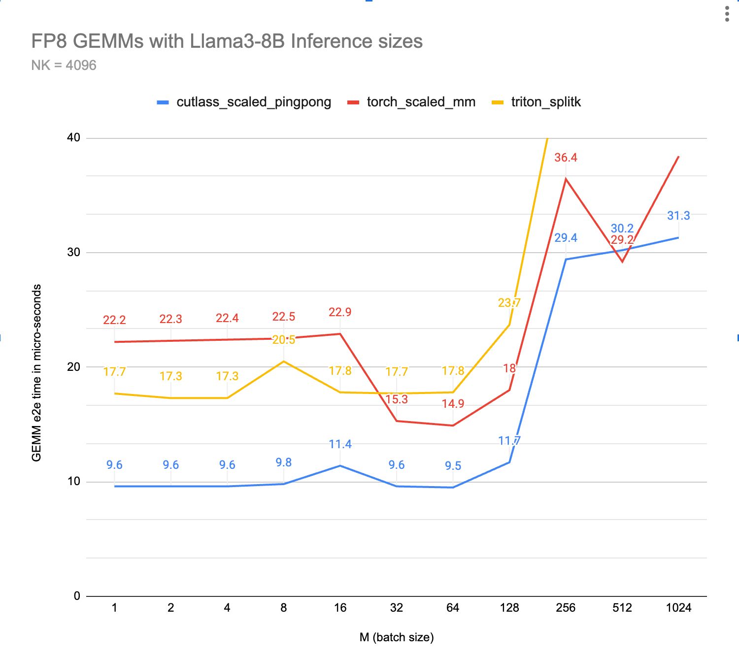
FlashAttention-3: Fast and Accurate Attention with Asynchrony and Low-precision

FlashAttention-3: Fast and Accurate Attention with Asynchrony and Low-precision

Attention, as a core layer of the ubiquitous Transformer architecture, is a bottleneck for large language models and long-context applications. FlashAttention (and FlashAttention-2) pioneered an approach to speed up attention on GPUs by minimizing memory reads/writes, and is now used by most libraries to accelerate Transformer training and inference. This has contributed to a massive increase in LLM context length in the last two years, from 2-4K (GPT-3, OPT) to 128K (GPT-4), or even 1M (Llama 3). However, despite its success, FlashAttention has yet to take advantage of new capabilities in modern hardware, with FlashAttention-2 achieving only 35% utilization of theoretical max FLOPs on the H100 GPU. In this blogpost, we describe three main techniques to speed up attention on Hopper GPUs: exploiting asynchrony of the Tensor Cores and TMA to (1) overlap overall computation and data movement via warp-specialization and (2) interleave block-wise matmul and softmax operations, and (3) incoherent processing that leverages hardware support for FP8 low-precision.

We’re excited to release FlashAttention-3 that incorporates these techniques. It’s 1.5-2.0x faster than FlashAttention-2 with FP16, up to 740 TFLOPS, i.e., 75% utilization of H100 theoretical max FLOPS. With FP8, FlashAttention-3 reaches close to 1.2 PFLOPS, with 2.6x smaller error than baseline FP8 attention.

FlashAttention-3 is available at: https://github.com/Dao-AILab/flash-attention
Paper

FlashAttention Recap

FlashAttention is an algorithm that reorders the attention computation and leverages tiling and recomputation to significantly speed it up and reduce memory usage from quadratic to linear in sequence length. We use tiling to load blocks of inputs from HBM (GPU memory) to SRAM (fast cache), perform attention with respect to that block, and update the output in HBM. By not writing the large intermediate attention matrices to HBM, we reduce the amount of memory reads/writes, which brings 2-4x wallclock time speedup.

Here we show a diagram of FlashAttention forward pass: with tiling and softmax rescaling, we operate by blocks and avoid having to read/write from HBM, while obtaining the correct output with no approximation.

math equations

New hardware features on Hopper GPUs – WGMMA, TMA, FP8

While FlashAttention-2 can achieve up to 70% theoretical max FLOPS on Ampere (A100) GPUs, it does not yet take advantage of new features on Hopper GPUs to maximize performance. We describe some of the new Hopper-specific features here, and why they are important.

1. WGMMA (Warpgroup Matrix Multiply-Accumulate). This new feature makes use of the new Tensor Cores on Hopper, with much higher throughput1 than the older mma.sync instruction in Ampere (image from the H100 white paper).

image from the H100 white paper

2. TMA (Tensor Memory Accelerator). This is a special hardware unit that accelerates the transfer of data between global memory and shared memory, taking care of all index calculation and out-of-bound predication. This frees up registers, which is a valuable resource to increase tile size and efficiency.

block diagram

3. Low-precision with FP8. This doubles the Tensor Core throughput (e.g. 989 TFLOPS with FP16 and 1978 TFLOPS with FP8), but trades off accuracy by using fewer bits to represent floating point numbers.

6x throughput

FlashAttention-3 makes use of all of these new features of Hopper, using powerful abstractions from NVIDIA’s CUTLASS library.

By rewriting FlashAttention to use these new features, we can already significantly speed it up (e.g., from 350 TFLOPS in FlashAttention-2 FP16 forward pass to around 540-570 TFLOPS). However, the asynchronous nature of the new instructions on Hopper (WGMMA and TMA) opens up additional algorithmic opportunities to overlap operations and thereby extract even greater performance. For this blogpost, we’ll explain two such techniques specific to attention. The generic technique of warp specialization, with separate producer and consumer warps doing TMA and WGMMA, is well-covered elsewhere in the context of GEMM and works the same here.

Asynchrony: Overlapping GEMM and Softmax

Why overlap?

Attention has GEMMs (those matmuls between Q and K and between attention probability P and V) and softmax as its two main operations. Why do we need to overlap them? Isn’t most of the FLOPS in the GEMMs anyway? As long as the GEMMs are fast (e.g., computed using WGMMA instructions), shouldn’t the GPU be going brrrr?

The problem is that non-matmul operations are much slower than matmul operations on modern accelerators. Special functions such as exponential (for the softmax) have even lower throughput than floating point multiply-add; they are evaluated by the multi-function unit, a unit separate from floating point multiply-add or matrix multiply-add. As an example, the H100 GPU SXM5 has 989 TFLOPS of FP16 matrix multiply, but only 3.9 TFLOPS (256x less throughput) for special functions2! For head dimension 128, there are 512x more matmul FLOPS than exponential, which means that exponential can take 50% of the time compared to matmul. The situation is even worse for FP8, where the matmul FLOPS are twice as fast yet exponential FLOPS stay the same speed. Ideally we want matmul and softmax to operate in parallel. While the Tensor Cores are busy with matmul, the multi-function units should be calculating exponential!

Inter-warpgroup overlapping with pingpong scheduling

The first and easiest way to overlap GEMM and softmax is to do nothing at all! The warp schedulers already try to schedule warps so that if some warps are blocked (e.g., waiting for GEMM results), other warps can run. That is, the warp schedulers do some of this overlapping for us, for free.

However, we can improve on this by doing some of the scheduling manually. As an example, if we have 2 warpgroups (labeled 1 and 2 – each warpgroup is a group of 4 warps), we can use synchronization barriers (bar.sync) so that warpgroup 1 first does its GEMMs (e.g., GEMM1 of one iteration and GEMM0 of the next iteration), and then warpgroup 2 does its GEMMs while warpgroup 1 does its softmax, and so on. This “pingpong” schedule is illustrated in the figure below, where the same color denotes the same iteration.

block chart

This would allow us to perform the softmax in the shadow of the GEMMs of the other warpgroup. Of course, this figure is just a caricature; in practice the scheduling is not really this clean. Nevertheless, pingpong scheduling can improve FP16 attention forward pass from around 570 TFLOPS to 620 TFLOPS (head dim 128, seqlen 8K).

Intra-warpgroup overlapping of GEMM and Softmax

Even within one warpgroup, we can have some part of softmax running while the GEMMs of that warpgroup is running. This is illustrated in this figure, where the same color denotes the same iteration.

block chart

This pipelining increases throughput from around 620 TFLOPS to around 640-660 TFLOPS for FP16 attention forward, at the cost of higher register pressure. We need more registers to hold both accumulators of the GEMMs, and the input/output of softmax. Overall, we find this technique to offer a favorable tradeoff.

Low-precision: reduce quantization error with incoherent processing

LLM activation can have outliers with much larger magnitude than the rest of the features. These outliers make it difficult to quantize, producing much larger quantization errors. We leverage incoherent processing, a technique used in the quantization literature (e.g. from QuIP) that multiplies the query and key with a random orthogonal matrix to “spread out” the outliers and reduce quantization error. In particular, we use the Hadamard transform (with random signs), which can be done per attention head in O(d log d) instead of O(d^2) time, where d is the head dimension. Since the Hadamard transform is memory-bandwidth bound, it can be fused with previous operations such as rotary embedding (also memory-bandwidth bound) “for free”.

In our experiment where Q, K, V are generated from a standard normal distribution but 0.1% of the entries have large magnitudes (to simulate outliers), we found that incoherent processing can reduce the quantization error by 2.6x. We show numerical error comparison in the table below. Please see the paper for details.

text diagram

Attention benchmark

We show some results with FlashAttention-3, and compare it to FlashAttention-2, as well as the implementation in Triton and cuDNN (both of which already use new hardware features of Hopper GPUs).

For FP16, we see about 1.6x-1.8x speedup over FlashAttention-2

speed charts

speed charts

For FP8, we can reach close to 1.2 PFLOPS!

speed charts

Discussion

This blogpost highlights some of the optimizations for FlashAttention available on Hopper GPUs. Other optimizations (e.g., variable length sequences, persistent kernel, and in-kernel transpose for FP8) are covered in the paper.

We have seen that designing algorithms that take advantage of the hardware they run on can bring significant efficiency gains and unlock new model capabilities such as long context. We look forward to future work on optimization for LLM inference, as well as generalizing our techniques to other hardware architectures.

We also look forward to FlashAttention-3 being integrated in a future release of PyTorch.

Notes

  1. Without the wgmma instruction, the older mma.sync instruction can only reach about ⅔ the peak throughput of Hopper Tensor Cores: https://arxiv.org/abs/2402.13499v1 

  2. The CUDA programming guide specifies that the throughput for special functions is 16 operations per streaming multiprocessor (SM) per clock cycle. We multiply 16 by 132 SMs and 1830 Mhz (clock speed used to calculate 989 TFLOPS of FP16 matmul) to get 3.9 TFLOPS 

Read More
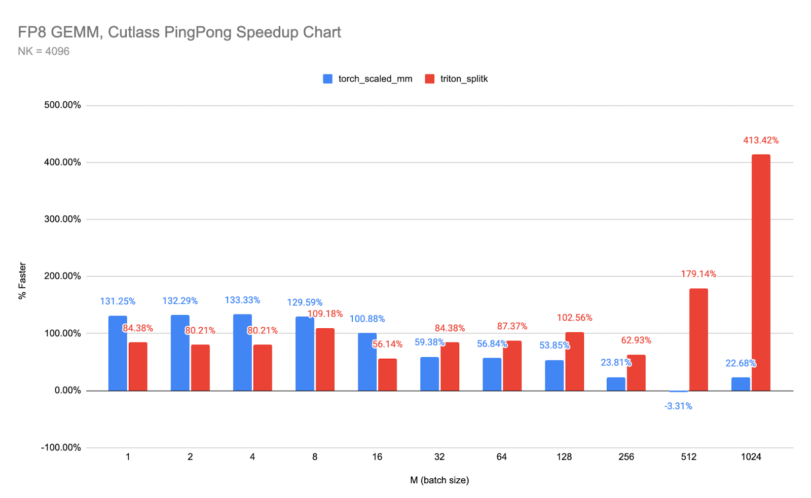
Learn how to develop Android applications with ExecuTorch and Llama models

This blog is courtesy of the PyTorch team at Arm. More details can be found here.

Arm’s compute platform is delivering GenAI applications on phones, laptops, and servers. Cost, privacy, performance, security, and energy efficiency are just some of the reasons developers are investigating on-device AI.

A new Learning Path explaining how to leverage the capabilities of large language models (LLMs) on Android using ExecuTorch and XNNPACK is now available.

Here’s a summary of what you’ll learn:

  • Development Environment setup

    The Learning Path begins by guiding you through setting up your development environment, ensuring you have all the necessary tools installed, including Android Studio, the Android NDK, Java JDK, and Python.

  • ExecuTorch and XNNPACK

    You’ll learn about the core technologies: ExecuTorch, a framework for deploying PyTorch models to edge devices, and XNNPACK, a high-performance library for executing neural networks on Arm-based platforms.

  • Llama models

    The Learning Path explores Llama, a family of powerful LLMs, focusing specifically on the 8B Llama 3 model. You’ll learn about quantization techniques, which are essential for optimizing model size and performance on mobile devices.

  • Prepare Llama models for ExecuTorch

    You’ll be guided through the process of downloading, exporting, and evaluating Llama models, ensuring they are ready for deployment using ExecuTorch.

  • Check model performance on Android

    The Learning Path walks you through cross-compiling the Llama runner binary for Android, allowing you to test your model’s performance on your phone.

  • Build and run an Android Chat App

    Finally, you’ll learn how to build a native Android chat app using the LlamaDemo application from the ExecuTorch repository. This hands-on experience allows you to put your knowledge into practice and create a real-world application.

Explore this Learning Path if you want to learn how to leverage the power of LLMs on your Android phone, and gain expertise in tools for on-device machine learning.

Dig into the excitement of building Android chat apps and understand more about how they work on the Arm Developer Hub.

Read More
Accelerated PyTorch inference with torch.compile on AWS Graviton processors

Accelerated PyTorch inference with torch.compile on AWS Graviton processors

Summary

Originally PyTorch, used an eager mode where each PyTorch operation that forms the model is run independently as soon as it’s reached. PyTorch 2.0 introduced torch.compile to speed up PyTorch code over the default eager mode. In contrast to eager mode, the torch.compile pre-compiles the entire model into a single graph in a manner that’s optimal for running on a given hardware platform. AWS optimized the PyTorch torch.compile feature for AWS Graviton3 processors. This optimization results in up to 2x better performance for Hugging Face model inference (based on geomean of performance improvement for 33 models) and up to 1.35x better performance for TorchBench model inference (geomean of performance improvement for 45 models) compared to the default eager mode inference across several natural language processing (NLP), computer vision (CV), and recommendation models on AWS Graviton3-based Amazon EC2 instances. Starting with PyTorch 2.3.1, the optimizations are available in torch Python wheels and AWS Graviton PyTorch deep learning container (DLC).

In this blog post, we show how we optimized torch.compile performance on AWS Graviton3-based EC2 instances, how to use the optimizations to improve inference performance, and the resulting speedups.

Why torch.compile and what’s the goal?

In eager mode, operators in a model are run immediately as they are encountered. It’s easier to use, more suitable for machine learning (ML) researchers, and hence is the default mode. However, eager mode incurs runtime overhead because of redundant kernel launch and memory read overhead. Whereas in torch compile mode, operators are first synthesized into a graph, wherein one operator is merged with another to reduce and localize memory reads and total kernel launch overhead.

The goal for the AWS Graviton team was to optimize torch.compile backend for Graviton3 processors. PyTorch eager mode was already optimized for Graviton3 processors with Arm Compute Library (ACL) kernels using oneDNN (also known as MKLDNN). So, the question was, how to reuse those kernels in torch.compile mode to get the best of graph compilation and the optimized kernel performance together?

Results

The AWS Graviton team extended the torch inductor and oneDNN primitives that reused the ACL kernels and optimized compile mode performance on Graviton3 processors. Starting with PyTorch 2.3.1, the optimizations are available in the torch Python wheels and AWS Graviton DLC. Please see the Running an inference section that follows for the instructions on installation, runtime configuration, and how to run the tests.

To demonstrate the performance improvements, we used NLP, CV, and recommendation models from TorchBench and the most downloaded NLP models from Hugging Face across Question Answering, Text Classification, Token Classification, Translation, Zero-Shot Classification, Translation, Summarization, Feature Extraction, Text Generation, Text2Text Generation, Fill-Mask, and Sentence Similarity tasks to cover a wide variety of customer use cases.

We started with measuring TorchBench model inference latency, in milliseconds (msec), for the eager mode, which is marked 1.0 with a red dotted line in the following graph. Then we compared the improvements from torch.compile for the same model inference, the normalized results are plotted in the graph. You can see that for the 45 models we benchmarked, there is a 1.35x latency improvement (geomean for the 45 models).

PyTorch model inference performance improvement with torch.compile on AWS Graviton3-based c7g instance using TorchBench framework

Image 1: PyTorch model inference performance improvement with torch.compile on AWS Graviton3-based c7g instance using TorchBench framework. The reference eager mode performance is marked as 1.0. (higher is better)

Similar to the preceding TorchBench inference performance graph, we started with measuring the Hugging Face NLP model inference latency, in msec, for the eager mode, which is marked 1.0 with a red dotted line in the following graph. Then we compared the improvements from torch.compile for the same model inference, the normalized results are plotted in the graph. You can see that for the 33 models we benchmarked, there is around 2x performance improvement (geomean for the 33 models).

Hugging Face NLP model inference performance improvement with torch.compile on AWS Graviton3-based c7g instance using Hugging Face example scripts

Image 2: Hugging Face NLP model inference performance improvement with torch.compile on AWS Graviton3-based c7g instance using Hugging Face example scripts. The reference eager mode performance is marked as 1.0. (higher is better)

Running an inference

Starting with PyTorch 2.3.1, the optimizations are available in the torch Python wheel and in AWS Graviton PyTorch DLC. This section shows how to run inference in eager and torch.compile modes using torch Python wheels and benchmarking scripts from Hugging Face and TorchBench repos.

To successfully run the scripts and reproduce the speedup numbers mentioned in this post, you need an instance from the Graviton3 family (c7g/r7g/m7g/hpc7g) of hardware. For this post, we used the c7g.4xl (16 vcpu) instance. The instance, the AMI details, and the required torch library versions are mentioned in the following snippet.

Instance: c7g.4xl instance
Region: us-west-2
AMI: ami-05cc25bfa725a144a (Ubuntu 22.04/Jammy with 6.5.0-1017-aws kernel)

# Install Python
sudo apt-get update
sudo apt-get install -y python3 python3-pip

# Upgrade pip3 to the latest version
python3 -m pip install --upgrade pip

# Install PyTorch and extensions
python3 -m pip install torch==2.3.1 torchvision==0.18.1 torchaudio==2.3.1

The generic runtime tunings implemented for eager mode inference are equally applicable for the torch.compile mode, so, we set the following environment variables to further improve the torch.compile performance on AWS Graviton3 processors.

# Enable the fast math GEMM kernels, to accelerate fp32 inference with bfloat16 gemm
export DNNL_DEFAULT_FPMATH_MODE=BF16

# Enable Linux Transparent Huge Page (THP) allocations,
# to reduce the tensor memory allocation latency
export THP_MEM_ALLOC_ENABLE=1

# Set LRU Cache capacity to cache the primitives and avoid redundant
# memory allocations
export LRU_CACHE_CAPACITY=1024

TORCHBENCH BENCHMARKING SCRIPTS

TorchBench is a collection of open source benchmarks used to evaluate PyTorch performance. We benchmarked 45 models using the scripts from the TorchBench repo. Following code shows how to run the scripts for the eager mode and the compile mode with inductor backend.

# Set OMP_NUM_THREADS to number of vcpus, 16 for c7g.4xl instance
export OMP_NUM_THREADS=16

# Install the dependencies
sudo apt-get install -y libgl1-mesa-glx
sudo apt-get install -y libpangocairo-1.0-0
python3 -m pip install psutil numpy transformers pynvml numba onnx onnxruntime scikit-learn timm effdet gym doctr opencv-python h5py==3.10.0 python-doctr 

# Clone pytorch benchmark repo
git clone https://github.com/pytorch/benchmark.git
cd benchmark
# PyTorch benchmark repo doesn't have any release tags. So,
# listing the commit we used for collecting the performance numbers
git checkout 9a5e4137299741e1b6fb7aa7f5a6a853e5dd2295

# Setup the models
python3 install.py 

# Colect eager mode performance using the following command. The results will be
# stored at .userbenchmark/cpu/metric-<timestamp>.json.
python3 run_benchmark.py cpu --model BERT_pytorch,hf_Bert,hf_Bert_large,hf_GPT2,hf_Albert,hf_Bart,hf_BigBird,hf_DistilBert,hf_GPT2_large,dlrm,hf_T5,mnasnet1_0,mobilenet_v2,mobilenet_v3_large,squeezenet1_1,timm_efficientnet,shufflenet_v2_x1_0,timm_regnet,resnet50,soft_actor_critic,phlippe_densenet,resnet152,resnet18,resnext50_32x4d,densenet121,phlippe_resnet,doctr_det_predictor,timm_vovnet,alexnet,doctr_reco_predictor,vgg16,dcgan,yolov3,pytorch_stargan,hf_Longformer,timm_nfnet,timm_vision_transformer,timm_vision_transformer_large,nvidia_deeprecommender,demucs,tts_angular,hf_Reformer,pytorch_CycleGAN_and_pix2pix,functorch_dp_cifar10,pytorch_unet --test eval --metrics="latencies,cpu_peak_mem"

# Collect torch.compile mode performance with inductor backend
# and weights pre-packing enabled. The results will be stored at
# .userbenchmark/cpu/metric-<timestamp>.json
python3 run_benchmark.py cpu --model BERT_pytorch,hf_Bert,hf_Bert_large,hf_GPT2,hf_Albert,hf_Bart,hf_BigBird,hf_DistilBert,hf_GPT2_large,dlrm,hf_T5,mnasnet1_0,mobilenet_v2,mobilenet_v3_large,squeezenet1_1,timm_efficientnet,shufflenet_v2_x1_0,timm_regnet,resnet50,soft_actor_critic,phlippe_densenet,resnet152,resnet18,resnext50_32x4d,densenet121,phlippe_resnet,doctr_det_predictor,timm_vovnet,alexnet,doctr_reco_predictor,vgg16,dcgan,yolov3,pytorch_stargan,hf_Longformer,timm_nfnet,timm_vision_transformer,timm_vision_transformer_large,nvidia_deeprecommender,demucs,tts_angular,hf_Reformer,pytorch_CycleGAN_and_pix2pix,functorch_dp_cifar10,pytorch_unet --test eval --torchdynamo inductor --freeze_prepack_weights --metrics="latencies,cpu_peak_mem"

On successful completion of the inference runs, the script stores the results in JSON format. The following is the sample output:

{
 "name": "cpu"
 "environ": {
     "pytorch_git_version": "d44533f9d073df13895333e70b66f81c513c1889"
  },
  
  "metrics": {
       "BERT_pytorch-eval_latency": 56.3769865,
       "BERT_pytorch-eval_cmem": 0.4169921875
  }
}

HUGGING FACE BENCHMARKING SCRIPTS

Google T5 Small Text Translation model is one of the around 30 Hugging Face models we benchmarked. We’re using it as a sample model to demonstrate how to run inference in eager and compile modes. The additional configurations and APIs required to run it in compile mode are highlighted in BOLD. Save the following script as google_t5_small_text_translation.py.

import argparse
from transformers import T5Tokenizer, T5Model
import torch
from torch.profiler import profile, record_function, ProfilerActivity
import torch._inductor.config as config
config.cpp.weight_prepack=True
config.freezing=True

def test_inference(mode, num_iter):
    tokenizer = T5Tokenizer.from_pretrained("t5-small")
    model = T5Model.from_pretrained("t5-small")

    input_ids = tokenizer(
        "Studies have been shown that owning a dog is good for you", return_tensors="pt"
    ).input_ids  # Batch size 1
    decoder_input_ids = tokenizer("Studies show that", return_tensors="pt").input_ids  # Batch size 1

    if (mode == 'compile'):
        model = torch.compile(model)

    with torch.no_grad():
        for _ in range(50):
            outputs = model(input_ids=input_ids, decoder_input_ids=decoder_input_ids)

        with profile(activities=[ProfilerActivity.CPU]) as prof:
            with record_function("model_inference"):
                for _ in range(num_iter):
                    outputs = model(input_ids=input_ids, decoder_input_ids=decoder_input_ids)

    print(prof.key_averages().table(sort_by="self_cpu_time_total"))

def main() -> None:
    global m, args
    parser = argparse.ArgumentParser(__doc__)
    parser.add_argument(
        "-m",
        "--mode",
        choices=["eager", "compile"],
        default="eager",
        help="Which test to run.",
    )
    parser.add_argument(
        "-n",
        "--number",
        type=int,
        default=100,
        help="how many iterations to run.",
    )
    args = parser.parse_args()
    test_inference(args.mode, args.number)

if __name__ == "__main__":
    main()

Run the script with the following steps:

# Set OMP_NUM_THREADS to number of vcpus to 4 because
# the scripts are running inference in sequence, and
# they don't need large number of vcpus
export OMP_NUM_THREADS=4

# Install the dependencies
python3 -m pip install transformers

# Run the inference script in Eager mode
# using number of iterations as 1 just to show the torch profiler output
# but for the benchmarking, we used 1000 iterations.
python3 google_t5_small_text_translation.py -n 1 -m eager

# Run the inference script in torch compile mode
python3 google_t5_small_text_translation.py -n 1 -m compile

On successful completion of the inference runs, the script prints the torch profiler output with the latency breakdown for the torch operators. The following is the sample output from torch profiler:

# Torch profiler output for the eager mode run on c7g.xl (4vcpu)
------------------------  ------------  ------------  ------------  ------------  ------------  ------------  
                    Name    Self CPU %      Self CPU   CPU total %     CPU total  CPU time avg    # of Calls  
------------------------  ------------  ------------  ------------  ------------  ------------  ------------  
                aten::mm        40.71%      12.502ms        40.71%      12.502ms     130.229us            96  
         model_inference        26.44%       8.118ms       100.00%      30.708ms      30.708ms             1  
               aten::bmm         6.85%       2.102ms         9.47%       2.908ms      80.778us            36  
            aten::matmul         3.73%       1.146ms        57.26%      17.583ms     133.205us           132  
            aten::select         1.88%     576.000us         1.90%     583.000us       0.998us           584  
         aten::transpose         1.51%     464.000us         1.83%     563.000us       3.027us           186  
------------------------ ------------ ------------ ------------ ------------ ------------ -------------------
Self CPU time total: 30.708ms

# Torch profiler output for the compile mode run for the same model on the same instance
---------------------------------  ------------  ------------  ------------  ------------  ------------  ------------  
                             Name    Self CPU %      Self CPU   CPU total %     CPU total  CPU time avg    # of Calls  
---------------------------------  ------------  ------------  ------------  ------------  ------------  ------------  
        mkldnn::_linear_pointwise        37.98%       5.461ms        45.91%       6.602ms      68.771us            96  
            Torch-Compiled Region        29.56%       4.251ms        98.53%      14.168ms      14.168ms             1  
                        aten::bmm        14.90%       2.143ms        21.73%       3.124ms      86.778us            36  
                     aten::select         4.51%     648.000us         4.62%     665.000us       1.155us           576  
                       aten::view         3.29%     473.000us         3.29%     473.000us       1.642us           288  
                      aten::empty         2.53%     364.000us         2.53%     364.000us       3.165us           115  
--------------------------------- ------------ ------------ ------------ ------------ ------------ --------------------
Self CPU time total: 14.379ms

Technical deep dive: What are the challenges and optimization details

Underpinning torch.compile are new technologies – TorchDynamo, AOTDispatcher, and TorchInductor.

TorchDynamo captures PyTorch programs safely using Python Frame Evaluation Hooks
AOTDispatcher overloads PyTorch’s autograd engine as a tracing autodiff for generating ahead-of-time backward traces.
TorchInductor is a deep learning compiler that generates fast code for multiple accelerators and backends.

The PyTorch compilation process source

Image 3: The PyTorch compilation process

When torch.compile is invoked, torch dynamo rewrites Python bytecode to extract sequences of PyTorch operations into an FX Graph, which is then compiled with inductor backend. For a typical inference scenario where the graph is frozen and gradient calculations are disabled, the inductor invokes platform specific optimizations like graph rewrite into more performant operators, operator fusion, and weights pre-packing.

However, on Graviton3, the inductor wasn’t able to perform any of those optimizations because there was no aarch64 backend defined. To fix this, we extended the inductor’s FX passes to pick oneDNN operators for linear layer compilation on Graviton3 processors with ACL backend. The code snippet for this follows:

packed_weight_op = (
    mkldnn._reorder_linear_weight
    if (is_bf16_weight or mkldnn._is_mkldnn_acl_supported())
                    
packed_linear_inputs: Tuple[Any, ...] = (input, packed_weight_node)
if is_bf16_weight or mkldnn._is_mkldnn_acl_supported():
    packed_linear_inputs += (bias, "none", [], "")
    packed_linear_op = mkldnn._linear_pointwise.default

After this was done, the FX pass was successful in compiling the matmul operators to linear_pointwise . The following snippet highlights the matmul operator in the original model:

 %attention_scores   : [num_users=1] = call_function[target=torch.matmul](args = (%query_layer, %transpose), kwargs = {})
 %attention_scores_1 : [num_users=1] = call_function[target=operator.truediv](args = (%attention_scores, 8.0), kwargs = {})
 %attention_scores_2 : [num_users=1] = call_function[target=operator.add](args = (%attention_scores_1, %extended_attention_mask_3), kwargs = {})

The following snippet highlights the linear_pointwise operator in the compiled graph:

%_linear_pointwise_default_140 : [num_users=2] = call_function[target=torch.ops.mkldnn._linear_pointwise.default](args = (%add_7, %_frozen_param278, %_frozen_param16, none, [], ), kwargs = {})
%mul_5 : [num_users=1] = call_function[target=torch.ops.aten.mul.Tensor](args = (%_linear_pointwise_default_140, 0.5), kwargs = {})
%mul_6 : [num_users=1] = call_function[target=torch.ops.aten.mul.Tensor](args = (%_linear_pointwise_default_140, 0.7071067811865476), kwargs = {})
%erf   : [num_users=1] = call_function[target=torch.ops.aten.erf.default](args = (%mul_6,), kwargs = {})
%add_8 : [num_users=1] = call_function[target=torch.ops.aten.add.Tensor](args = (%erf, 1), kwargs = {})

This completes the torch inductor changes required to compile the graph into optimized operators on AWS Graviton3 processors. Next comes the actual inference where the compiled graph is dispatched to be run. OneDNN with ACL was the backend we chose during the inductor compilation, so, the new operators were dispatched to oneDNN as expected, for example, mkldnn._linear_pointwise. However, due to gaps in oneDNN ACL primitives, the operators were run with C++ reference kernels instead of the optimized ACL kernels. Hence, the compile performance was still significantly behind the eager mode performance.

There were mainly three areas where oneDNN ACL primitives lack support for torch.compile mode. The following section talks about them in detail.

1 ACL primitives didn’t have support for weights in blocked layout

ACL primitives originally designed for eager mode supported weights only in the standard channels last (NHWC) format, without any pre-packing. Whereas weights pre-packing into blocked layout is one of the main optimizations in the inductor compilation passes where the weights are reordered into blocks specific to the runtime platform. This avoids the redundant and on-the-fly reorders when running the General Matrix Multiplication (GEMM), which otherwise would be the bottleneck for inference performance. But the ACL primitives didn’t have support for blocked layout and hence the operators were run with oneDNN C++ reference kernels instead.

2 Mixed precision primitives weren’t supported in oneDNN

AWS Graviton3 processors support bfloat16 MMLA instructions which can be used to accelerate fp32 inference with bfloat16 GEMM as a mixed precision compute. ACL supports bfloat16 mixed precision GEMM kernels, and are integrated into oneDNN as a fast math compute option for the existing fp32 operators. However, the fast math approach didn’t work for compile mode because of weights pre-packing optimization. The compile mode requires explicit mixed precision primitive implementation in oneDNN in order to use bfloat16 acceleration.

3 ACL primitives didn’t support fused kernels for some of the activation functions

In eager mode, operators are dispatched individually because the model is run independently as soon as it’s reached. Whereas in compile mode, operator fusion is another important optimization where the operators are fused for runtime efficiency. For example, Gaussian Error Linear Unit (GELU) is one of the most widely used activation functions in transformers-based neural network architectures. So, it’s typical to have a linear layer (with matrix multiplications) followed by GELU activation. As part of compiling the model into efficient operators, the torch inductor fuses matmul and GELU into a single linearpointwise+gelu operator. However, oneDNN ACL primitives didn’t have the support for fused kernels with GELU.

We addressed these gaps by extending oneDNN primitives to handle the additional layouts and new primitive definitions. The following sections talk about the optimizations in detail.

Optimization 1: Extended ACL primitives to accept weight tensors in blocked layout

We extended the ACL primitives to accept blocked layout in addition to the the standard NHWC format. The code snippet for this is as follows:

const bool is_weights_md_format_ok
                    = utils::one_of(weights_format_kind_received,
                      format_kind::any, format_kind::blocked);


const memory_desc_t weights_md_received = weights_md_;
acl_utils::reorder_to_weight_format(aip.wei_tensor_info,
             weights_md_, expected_weight_format, inner_dim, o_dim,
             remaining_dims, {});

ACL_CHECK_SUPPORT(
     (weights_format_kind_received == format_kind::blocked)
      && !(dnnl_memory_desc_equal(
      &weights_md_received, &weights_md_)),
      "specified blocked format not supported by ACL, use "
      "format_kind_t::any to find a supported blocked format for "
      "your platform");

Optimization 2: Defined new ACL primitives to handle mixed precision operators (weights in bfloat16 and activations in fp32)

We defined mixed precision primitive definitions and updated the existing oneDNN ACL fp32 primitives to handle bfloat16 tensors.

 /* With graph compilation, we are able to reorder and pre-pack the weights during the model load
  * and compilation phase itself so that redundant and on-the-fly reorders can be avoided.
  * This primitive definition is to support gemm fastmath mode for the compile scenario where src is
  * in fp32 and weights are in bf16
  */
 {{forward, f32, bf16, f32}, {
    CPU_INSTANCE_AARCH64_ACL(acl_inner_product_fwd_t)
    nullptr,
 }},

Optimization 3: Disabled operator fusion pass in torch inductor

We bypassed the operator fusion pass in torch inductor so that the compiled graph doesn’t contain GELU fused operators. This is a temporary solution to enable ACL kernels in torch.compile. There is a work in progress to enable operator fusion pass for the future PyTorch releases. With this workaround, we were able to successfully dispatch the linear layer to ACL. As shown in the following torch.profiler output, the aten::addmm (one of the variants of the matmul operator) and aten::gelu in the original model (as highlighted in Image 4) was compiled to mkldnn::_linear_pointwise without gelu operator fusion (as highlighted in Image 5).

---------------------------  ------------  ------------  ------------  ------------  ------------  ------------  
                       Name    Self CPU %      Self CPU   CPU total %     CPU total  CPU time avg    # of Calls  
---------------------------  ------------  ------------  ------------  ------------  ------------  ------------  
                aten::addmm        73.32%      46.543ms        74.49%      47.287ms     647.767us            73  
            model_inference         9.92%       6.296ms       100.00%      63.479ms      63.479ms             1  
                  aten::bmm         4.37%       2.776ms         5.46%       3.467ms     144.458us            24  
                aten::copy_         1.74%       1.102ms         1.74%       1.102ms       8.103us           136  
                 aten::gelu         1.50%     950.000us         1.50%     950.000us      79.167us            12  

Image 4: torch.profiler output for Hugging Face bert base model inference in Eager mode, showing addmm and gelu operators

 
-----------------------------------------------------  ------------  ------------  ------------  ------------  ------------  ------------  
                                                 Name    Self CPU %      Self CPU   CPU total %     CPU total  CPU time avg    # of Calls  
-----------------------------------------------------  ------------  ------------  ------------  ------------  ------------  ------------  
                            mkldnn::_linear_pointwise        53.61%      15.529ms        57.53%      16.665ms     228.288us            73  
                                Torch-Compiled Region        36.95%      10.705ms        99.31%      28.769ms      28.769ms             1  
    aten::_scaled_dot_product_flash_attention_for_cpu         3.67%       1.064ms         4.43%       1.284ms     107.000us            12  
                                           aten::view         1.97%     572.000us         1.97%     572.000us       2.509us           228  
                                          aten::empty         1.38%     399.000us         1.38%     399.000us       3.270us           122 

Image 5: torch.profiler output for Hugging Face Bert base model inference in torch.compile mode, showing linear_pointwise operator without gelu fusion

Lastly, the gelu operator was compiled into erf (error function) and was dispatched to an inductor auto vectorization backend. The following snippets show the erf operator in the compiled graph and running it using libm.so.

%_linear_pointwise_default_140 : [num_users=2] = call_function[target=torch.ops.mkldnn._linear_pointwise.default](args = (%add_7, %_frozen_param278, %_frozen_param16, none, [], ), kwargs = {})
%mul_5 : [num_users=1] = call_function[target=torch.ops.aten.mul.Tensor](args = (%_linear_pointwise_default_140, 0.5), kwargs = {})
%mul_6 : [num_users=1] = call_function[target=torch.ops.aten.mul.Tensor](args = (%_linear_pointwise_default_140, 0.7071067811865476), kwargs = {})
%erf   : [num_users=1] = call_function[target=torch.ops.aten.erf.default](args = (%mul_6,), kwargs = {})
%add_8 : [num_users=1] = call_function[target=torch.ops.aten.add.Tensor](args = (%erf, 1), kwargs = {})

Image 6: snippet after post grad pass showing erf function in the compiled graph

 
     0.82%     0.40%  python3  libm.so.6            [.] erff32
     0.05%     0.00%  python3  libtorch_python.so   [.] torch::autograd::THPVariable_erf
     0.05%     0.00%  python3  libtorch_cpu.so      [.] at::_ops::erf::call

Image 7: Linux perf report showing erf dispatch to libm.so

With this work, we were able to optimize torch.compile performance on Graviton3 processors by using inductor graph compilation along with the oneDNN+ACL backend.

TorchBench enhancements

To demonstrate the torch.compile performance improvements on AWS Graviton3 processors, we extended TorchBench framework to add a new argument to enable graph freeze and weights pre-packing and disable torch auto grad for eval test mode. The code snippet for this is as follows:

parser.add_argument(
 "—freeze_prepack_weights",
 action='store_true',
 help="set to freeze the graph and prepack weights",
 )

if args.freeze_prepack_weights:
 torch._inductor.config.freezing=True
 torch._inductor.config.cpp.weight_prepack=True

Image 8: Added freeze_prepack_weights option for torchdynamo backend in TorchBench to demonstrate torch.compile performance improvements on AWS Graviton3 processors

We have upstreamed all the optimizations, and starting with PyTorch 2.3.1, these are supported in torch Python wheels and AWS Graviton PyTorch DLC.

What’s next

Next, we’re extending the torch inductor CPU backend support to compile Llama model, and adding support for fused GEMM kernels to enable torch inductor operator fusion optimization on AWS Graviton3 processors.

Conclusion

In this tutorial, we covered how we optimized torch.compile performance on AWS Graviton3-based EC2 instances, how to use the optimizations to improve PyTorch model inference performance, and demonstrated the resulting speedups. We hope that you will give it a try! If you need any support with ML software on Graviton, please open an issue on the AWS Graviton Technical Guide GitHub.

Acknowledgements

We would like to thank the PyTorch community for the baseline torch.compile framework and their continued efforts to optimize it further.

Author

Sunita Nadampalli is a Software Development Manager and AI/ML expert at AWS. She leads AWS Graviton software performance optimizations for AI/ML and HPC workloads. She is passionate about open source software development and delivering high-performance and sustainable software solutions for SoCs based on the Arm ISA.

Read More
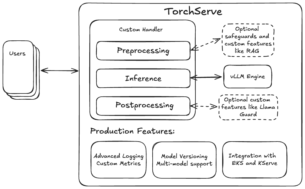
Announcing Hacker Cup AI Track at NeurIPS 2024

The PyTorch team in partnership with Meta Hacker Cup, and Microsoft Research, are excited to announce the Hacker Cup AI Track at NeurIPS 2024. This will be the first AI track for the popular Meta Hacker Cup programming competition designed to assess the capabilities of Generative AI in performing autonomous code generation tasks. We aim to test the limits of AI in complex coding challenges and measure the performance gap between AI systems and human programmers. We will provide access to all Hacker Cup problems since 2011 alongside their respective solutions in a multimodal (image and text) format, and utilize the existing Hacker Cup infrastructure for competitor evaluation. Featuring both open evaluation, open model and open evaluation, closed model tracks, this competition invites diverse participation from research institutions of varied interests and resource constraints, including academic labs, AI startups, large technology companies, and AI enthusiasts. Our goal is to develop and democratize meaningful advancements in code automation with the very first open evaluation process for competitive AI programmers. Registration will begin in Early August, with our first qualification round on September 20th.

For more information please visit our website at https://www.facebook.com/codingcompetitions/hacker-cup/ and join our Discord at discord.gg/wWeN9hTH32
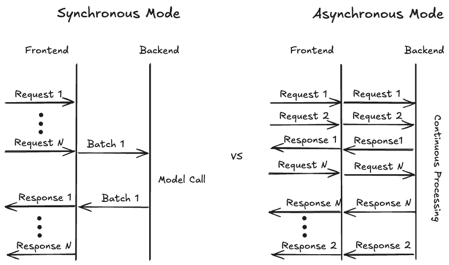
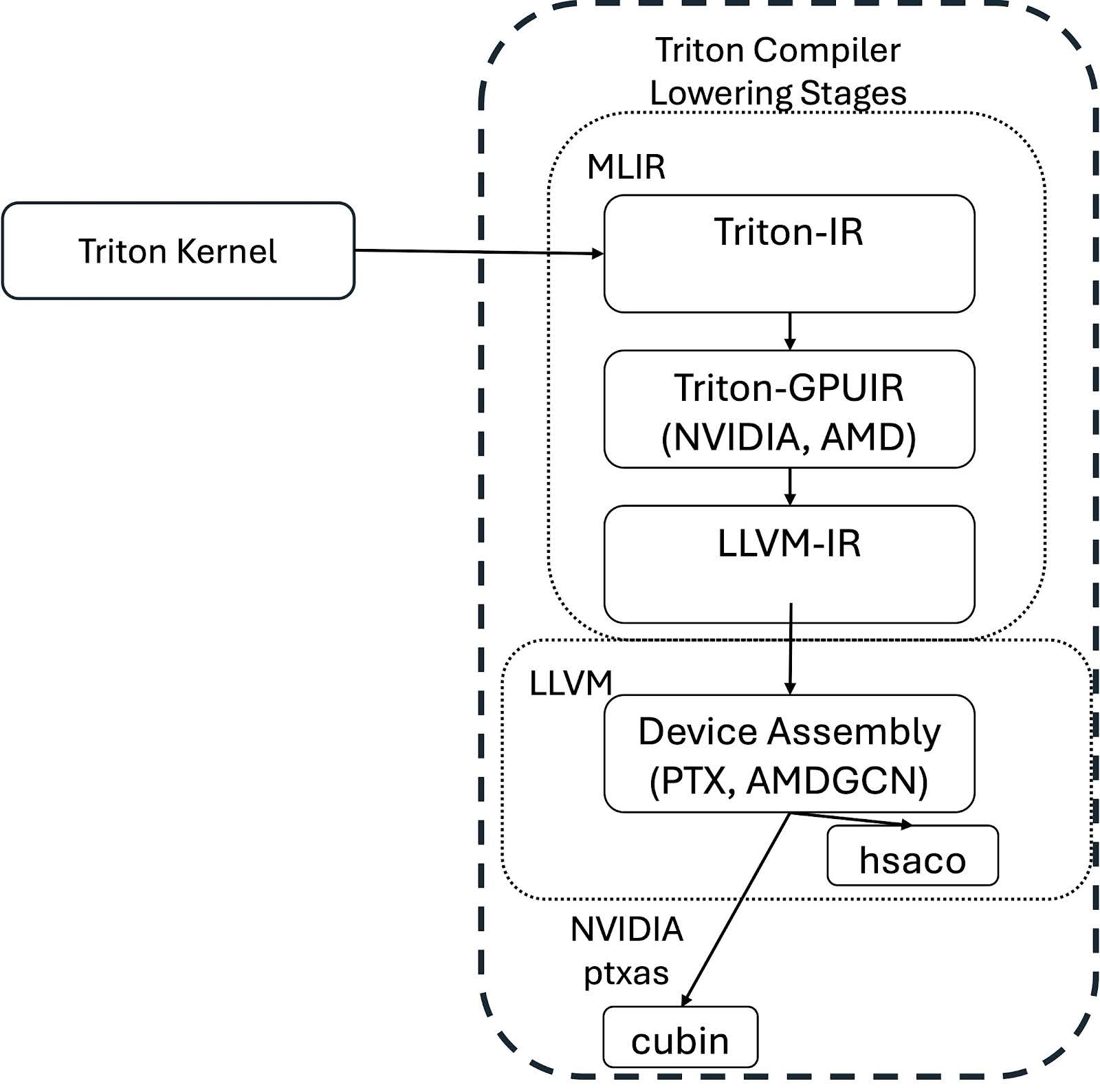
Read More