Create high-quality datasets with Amazon SageMaker Ground Truth and FiftyOne

This is a joint post co-written by AWS and Voxel51. Voxel51 is the company behind FiftyOne, the open-source toolkit for building high-quality datasets and computer vision models.

A retail company is building a mobile app to help customers buy clothes. To create this app, they need a high-quality dataset containing clothing images, labeled with different categories. In this post, we show how to repurpose an existing dataset via data cleaning, preprocessing, and pre-labeling with a zero-shot classification model in FiftyOne, and adjusting these labels with Amazon SageMaker Ground Truth.

You can use Ground Truth and FiftyOne to accelerate your data labeling project. We illustrate how to seamlessly use the two applications together to create high-quality labeled datasets. For our example use case, we work with the Fashion200K dataset, released at ICCV 2017.

Solution overview

Ground Truth is a fully self-served and managed data labeling service that empowers data scientists, machine learning (ML) engineers, and researchers to build high-quality datasets. FiftyOne by Voxel51 is an open-source toolkit for curating, visualizing, and evaluating computer vision datasets so that you can train and analyze better models by accelerating your use cases.

In the following sections, we demonstrate how to do the following:

• Visualize the dataset in FiftyOne
• Clean the dataset with filtering and image deduplication in FiftyOne
• Pre-label the cleaned data with zero-shot classification in FiftyOne
• Label the smaller curated dataset with Ground Truth
• Inject labeled results from Ground Truth into FiftyOne and review labeled results in FiftyOne

Use case overview

Suppose you own a retail company and want to build a mobile application to give personalized recommendations to help users decide what to wear. Your prospective users are looking for an application that tells them which articles of clothing in their closet work well together. You see an opportunity here: if you can identify good outfits, you can use this to recommend new articles of clothing that complement the clothing a customer already owns.

You want to make things as easy as possible for the end-user. Ideally, someone using your application only needs to take pictures of the clothes in their wardrobe, and your ML models work their magic behind the scenes. You might train a general-purpose model or fine-tune a model to each user’s unique style with some form of feedback.

First, however, you need to identify what type of clothing the user is capturing. Is it a shirt? A pair of pants? Or something else? After all, you probably don’t want to recommend an outfit that has multiple dresses or multiple hats.

To address this initial challenge, you want to generate a training dataset consisting of images of various articles of clothing with various patterns and styles. To prototype with a limited budget, you want to bootstrap using an existing dataset.

To illustrate and walk you through the process in this post, we use the Fashion200K dataset released at ICCV 2017. It’s an established and well-cited dataset, but it isn’t directly suited for your use case.

Although articles of clothing are labeled with categories (and subcategories) and contain a variety of helpful tags that are extracted from the original product descriptions, the data is not systematically labeled with pattern or style information. Your goal is to turn this existing dataset into a robust training dataset for your clothing classification models. You need to clean the data, augmenting the labeling schema with style labels. And you want to do so quickly and with as little spend as possible.

Download the data locally

First, download the women.tar zip file and the labels folder (with all of its subfolders) following the instructions provided in the Fashion200K dataset GitHub repository. After you’ve unzipped them both, create a parent directory fashion200k, and move the labels and women folders into this. Fortunately, these images have already been cropped to the object detection bounding boxes, so we can focus on classification, rather than worry about object detection.

Despite the “200K” in its moniker, the women directory we extracted contains 338,339 images. To generate the official Fashion200K dataset, the dataset’s authors crawled more than 300,000 products online, and only products with descriptions containing more than four words made the cut. For our purposes, where the product description isn’t essential, we can use all of the crawled images.

Let’s look at how this data is organized: within the women folder, images are arranged by top-level article type (skirts, tops, pants, jackets, and dresses), and article type subcategory (blouses, t-shirts, long-sleeved tops).

Within the subcategory directories, there is a subdirectory for each product listing. Each of these contains a variable number of images. The cropped_pants subcategory, for instance, contains the following product listings and associated images.

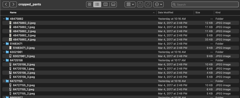
The labels folder contains a text file for each top-level article type, for both train and test splits. Within each of these text files is a separate line for each image, specifying the relative file path, a score, and tags from the product description.

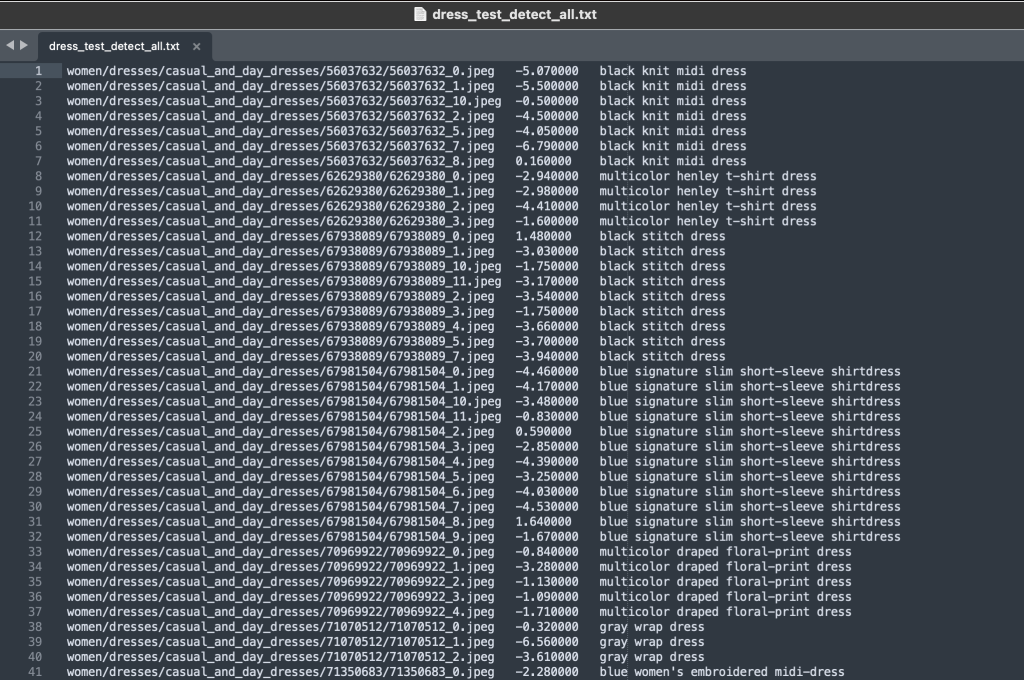
Because we’re repurposing the dataset, we combine all of the train and test images. We use these to generate a high-quality application-specific dataset. After we complete this process, we can randomly split the resulting dataset into new train and test splits.

Inject, view, and curate a dataset in FiftyOne

If you haven’t already done so, install open-source FiftyOne using pip:

pip install fiftyone

A best practice is to do so within a new virtual (venv or conda) environment. Then import the relevant modules. Import the base library, fiftyone, the FiftyOne Brain, which has built-in ML methods, the FiftyOne Zoo, from which we will load a model that will generate zero-shot labels for us, and the ViewField, which lets us efficiently filter the data in our dataset:

import fiftyone as fo
import fiftyone.brain as fob
import fiftyone.zoo as foz
from fiftyone import ViewField as F

You also want to import the glob and os Python modules, which will help us work with paths and pattern match over directory contents:

from glob import glob
import os

Now we’re ready to load the dataset into FiftyOne. First, we create a dataset named fashion200k and make it persistent, which allows us to save the results of computationally intensive operations, so we only need to compute said quantities once.

dataset = fo.Dataset("fashion200k", persistent=True)

We can now iterate through all subcategory directories, adding all the images within the product directories. We add a FiftyOne classification label to each sample with the field name article_type, populated by the image’s top-level article category. We also add both category and subcategory information as tags:

# Map dir categories to article type labels
labels_map = {
    "dresses": "dress",
    "jackets": "jacket",
    "pants": "pants",
    "skirts": "skirt",
    "tops": "top",
}

dataset_dir = "./fashion200k"

for d in glob(os.path.join(dataset_dir, "women", "*", "*")):
    _, _, category, subcategory = d.split("/")
    subcategory = subcategory.replace("_", " ")
    label = labels_map[category]

    dataset.add_samples(
        [
            fo.Sample(
                    filepath=filepath,
tags=[category, subcategory],   article_type=fo.Classification(label=label),
            )
            for filepath in glob(os.path.join(d, "*", "*"))
        ]
    )

At this point, we can visualize our dataset in the FiftyOne app by launching a session:

session = fo.launch_app(dataset)

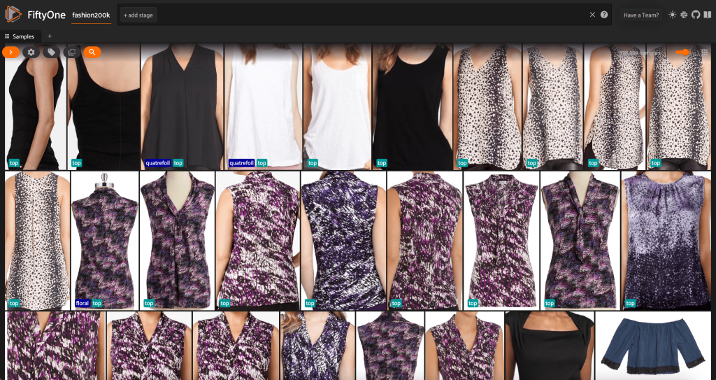
We can also print out a summary of the dataset in Python by running print(dataset):

Name:        fashion200k
Media type:  image
Num samples: 338339
Persistent:  True
Tags:        []
Sample fields:
    id:            fiftyone.core.fields.ObjectIdField
    filepath:      fiftyone.core.fields.StringField
    tags:          fiftyone.core.fields.ListField(fiftyone.core.fields.StringField)
    metadata:      fiftyone.core.fields.EmbeddedDocumentField(fiftyone.core.metadata.ImageMetadata)
    article_type:  fiftyone.core.fields.EmbeddedDocumentField(fiftyone.core.labels.Classification)

We can also add the tags from the labels directory to the samples in our dataset:

working_dir = os.getcwd()

tags = {
f: set(t) 
for f, t in zip(*dataset.values(["filepath", "tags"]))
}


for label_file in glob("fashion200k/labels/*"):
    with open(label_file, 'r') as f:
        for line in f.readlines():
            line_list = line.split()
            fp = os.path.join(
                working_dir, 
                dataset_dir, 
                line_list[0]
            )
          
           # add new tags
          new_tags_for_fp = line_list[2:]
          tags[fp].update(new_tags_for_fp)

# Update tags
dataset.set_values("tags", tags, key_field="filepath")

Looking at the data, a few things become clear:

• Some of the images are fairly grainy, with low resolution. This is likely because these images were generated by cropping initial images in object detection bounding boxes.
• Some clothes are worn by a person, and some are photographed on their own. These details are encapsulated by the viewpoint property.
• A lot of the images of the same product are very similar, so at least initially, including more than one image per product may not add much predictive power. For the most part, the first image of each product (ending in _0.jpeg) is the cleanest.

Initially, we might want to train our clothing style classification model on a controlled subset of these images. To this end, we use high-resolution images of our products, and limit our view to one representative sample per product.

First, we filter out the low-resolution images. We use the compute_metadata() method to compute and store image width and height, in pixels, for each image in the dataset. We then employ the FiftyOne ViewField to filter out images based on the minimum allowed width and height values. See the following code:

dataset.compute_metadata()

min_width = 200
min_height = 300

width_filter = F("metadata.width") > min_width
height_filter = F("metadata.height") > min_height


high_res_view = dataset.match(
    width_filter & height_filter
)

session.view = high_res_view.view()

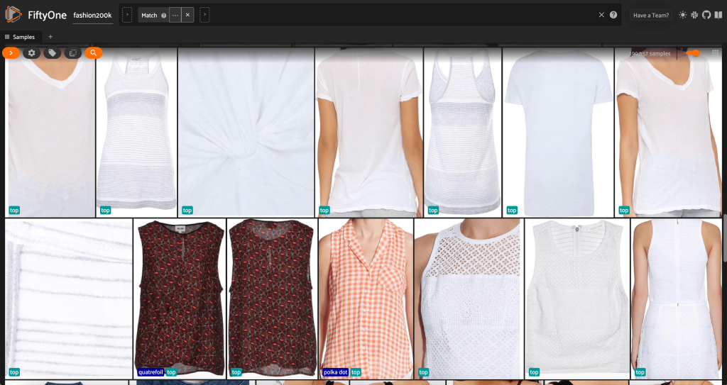
This high-resolution subset has just under 200,000 samples.

From this view, we can create a new view into our dataset containing only one representative sample (at most) for each product. We use the ViewField once again, pattern matching for file paths that end with _0.jpeg:

representative_view = high_res_view.match(
    F("filepath").ends_with("_0.jpeg")
)

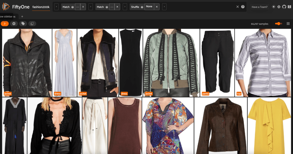
Let’s view a randomly shuffled ordering of images in this subset:

session.view = representative_view.shuffle()

Remove redundant images in the dataset

This view contains 66,297 images, or just over 19% of the original dataset. When we look at the view, however, we see that there are many very similar products. Keeping all of these copies will likely only add cost to our labeling and model training, without noticeably improving performance. Instead, let’s get rid of the near duplicates to create a smaller dataset that still packs the same punch.

Because these images are not exact duplicates, we can’t check for pixel-wise equality. Fortunately, we can use the FiftyOne Brain to help us clean our dataset. In particular, we’ll compute an embedding for each image—a lower-dimensional vector representing the image—and then look for images whose embedding vectors are close to each other. The closer the vectors, the more similar the images.

We use a CLIP model to generate a 512-dimensional embedding vector for each image, and store these embeddings in the field embeddings on the samples in our dataset:

## load model
model = foz.load_zoo_model("clip-vit-base32-torch")
 
## compute embeddings
representative_view.compute_embeddings(
model, 
embeddings_field="embedding"
)

Then we compute the closeness between embeddings, using cosine similarity, and assert that any two vectors whose similarity is greater than some threshold are likely to be near duplicates. Cosine similarity scores lie in the range [0, 1], and looking at the data, a threshold score of thresh=0.5 seems to be about right. Again, this doesn’t need to be perfect. A few near-duplicate images are not likely to ruin our predictive power, and throwing away a few non-duplicate images doesn’t materially impact model performance.

results = fob.compute_similarity(
view,
embeddings="embedding",
brain_key="sim",
metric="cosine"
)

results.find_duplicates(thresh=0.5)

We can view the purported duplicates to verify that they are indeed redundant:

## view the duplicates, paired up, 
## to make sure it is doing what we think it is doing
dup_view = results.duplicates_view()
session = fo.launch_app(dup_view)

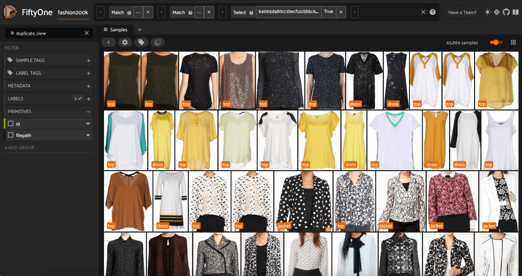
When we’re happy with the result and believe these images are indeed near duplicates, we can pick one sample from each set of similar samples to keep, and ignore the others:

## get one image from each group of duplicates
dup_rep_ids = list(results.neighbors_map.keys())

# get ids of non-duplicates
non_dup_ids = representative_view.exclude(
dup_view.values("id")
).values("id")

# ids to keep
ids = dup_rep_ids + non_dup_ids

# create view from ids
non_dup_view = representative_view[ids]

Now this view has 3,729 images. By cleaning the data and identifying a high-quality subset of the Fashion200K dataset, FiftyOne lets us restrict our focus from more than 300,000 images to just under 4,000, representing a reduction by 98%. Using embeddings to remove near-duplicate images alone brought our total number of images under consideration down by more than 90%, with little if any effect on any models to be trained on this data.

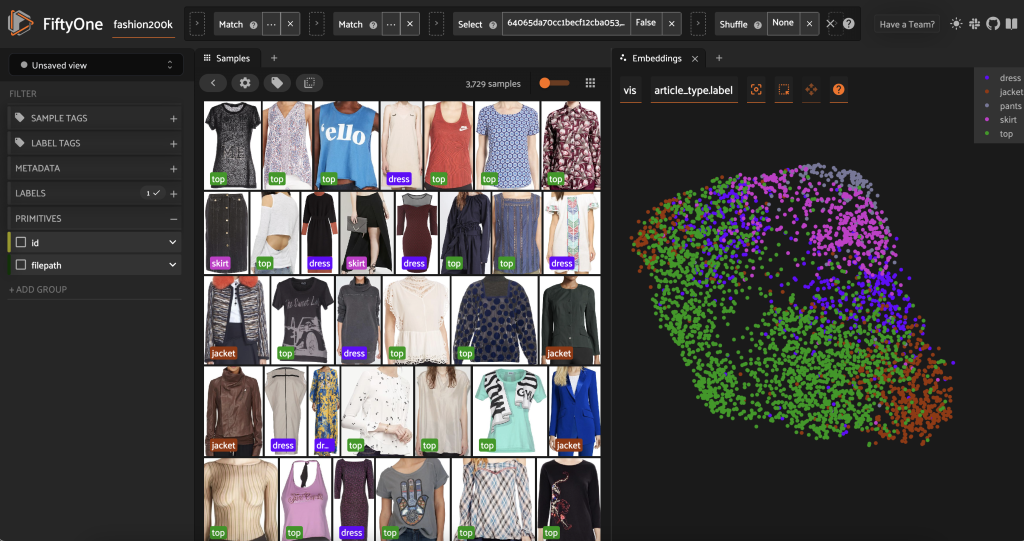
Before pre-labeling this subset, we can better understand the data by visualizing the embeddings we have already computed. We can use the FiftyOne Brain’s built-in compute_visualization() method, which employs the uniform manifold approximation (UMAP) technique to project the 512-dimensional embedding vectors into two-dimensional space so we can visualize them:

fob.compute_visualization(
    non_dup_view, 
    embeddings="embedding", 
    brain_key="vis"
)

We open a new Embeddings panel in the FiftyOne app and coloring by article type, and we can see that these embeddings roughly encode a notion of article type (among other things!).

Now we are ready to pre-label this data.

Inspecting these highly unique, high-resolution images, we can generate a decent initial list of styles to use as classes in our pre-labeling zero-shot classification. Our goal in pre-labeling these images is not to necessarily label each image correctly. Rather, our goal is to provide a good starting point for human annotators so we can reduce labeling time and cost.

styles = [
 "graphic", 
 "lettered", 
 "plain", 
 "striped", 
 "polka dot", 
 "floral", 
 "jersey", 
 "checkered", 
 "denim", 
 "plaid",
 "houndstooth",
 "chevron", 
 "paisley", 
 "animal print", 
 "quatrefoil",
 “camouflage”
]

We can then instantiate a zero-shot classification model for this application. We use a CLIP model, which is a general-purpose model trained on both images and natural language. We instantiate a CLIP model with the text prompt “Clothing in the style,” so that given an image, the model will output the class for which “Clothing in the style [class]” is the best fit. CLIP is not trained on retail or fashion-specific data, so this won’t be perfect, but it can save you in labeling and annotation costs.

zero_shot_model = foz.load_zoo_model(
 "clip-vit-base32-torch",
 text_prompt="Clothing in the style ",
 classes=styles,
)

We then apply this model to our reduced subset and store the results in an article_style field:

non_dup_view.apply_model(
zero_shot_model, 
label_field="article_style"
)

Launching the FiftyOne App once again, we can visualize the images with these predicted style labels. We sort by prediction confidence so we view the most confident style predictions first:

high_conf_view = non_dup_view.sort_by(
 "article_style.confidence", reverse=True
)

session.view = high_conf_view

We can see that the highest confidence predictions seem to be for “jersey,” “animal print,” “polka dot,” and “lettered” styles. This makes sense, because these styles are relatively distinct. It also seems like, for the most part, the predicted style labels are accurate.

We can also look at the lowest-confidence style predictions:

low_conf_view = non_dup_view.sort_by(
"article_style.confidence"
)
session.view = low_conf_view

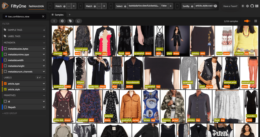
For some of these images, the appropriate style category is in the provided list, and the article of clothing is incorrectly labeled. The first image in the grid, for instance, should clearly be “camouflage” and not “chevron.” In other cases, however, the products don’t fit neatly into the style categories. The dress in the second image in the second row, for example, is not exactly “striped,” but given the same labeling options, a human annotator might also have been conflicted. As we build out our dataset, we need to decide whether to remove edge cases like these, add new style categories, or augment the dataset.

Export the final dataset from FiftyOne

Export the final dataset with the following code:

# The directory to which to write the exported dataset
export_dir = "200kFashionDatasetExportResult"

# The name of the sample field containing the label that you wish to export
# Used when exporting labeled datasets (e.g., classification or detection)
label_field = "article_style"  # for example

# The type of dataset to export
# Any subclass of `fiftyone.types.Dataset` is supported
dataset_type = fo.types.COCODetectionDataset  # for example

# Export the dataset
high_conf_view.export(
    export_dir=export_dir,
    dataset_type=dataset_type,
    label_field=label_field,
)

We can export a smaller dataset, for example, 16 images, to the folder 200kFashionDatasetExportResult-16Images. We create a Ground Truth adjustment job using it:

# The directory to which to write the exported dataset
export_dir = "200kFashionDatasetExportResult-16Images"

# The name of the sample field containing the label that you wish to export
# Used when exporting labeled datasets (e.g., classification or detection)
label_field = "article_style"  # for example

# The type of dataset to export
# Any subclass of `fiftyone.types.Dataset` is supported
dataset_type = fo.types.COCODetectionDataset  # for example

# Export the dataset
high_conf_view.take(16).export(
    export_dir=export_dir,
    dataset_type=dataset_type,
    label_field=label_field,
)

Upload the revised dataset, convert the label format to Ground Truth, upload to Amazon S3, and create a manifest file for the adjustment job

We can convert the labels in the dataset to match the output manifest schema of a Ground Truth bounding box job, and upload the images to an Amazon Simple Storage Service (Amazon S3) bucket to launch a Ground Truth adjustment job:

import json
# open the labels.json file of ground truth bounding box 
#labels from the exported dataset
f = open('200kFashionDatasetExportResult-16Images/labels.json')
data = json.load(f)

# provide your aws s3 bucket name, prefix, and aws credentials
bucket_name = 'sagemaker-your-preferred-s3-bucket'
s3_prefix = 'sagemaker-your-preferred-s3-prefix'

session = boto3.Session(
    aws_access_key_id='<AWS_ACCESS_KEY_ID>',
    aws_secret_access_key='<AWS_SECRET_ACCESS_KEY>'
)
s3 = session.resource('s3')

for image in data['images']:
    file_name = image['file_name']
    file_id = file_name[:-4]
    image_id = image['id']
    
    # upload the image to s3
    s3.meta.client.upload_file('200kFashionDatasetExportResult-16Images/data/'+image['file_name'], bucket_name, s3_prefix+'/'+image['file_name'])
    
    gt_annotations = []
    confidence = 0.00
    
    for annotation in data['annotations']:
        if annotation['image_id'] == image['id']:
            confidence = annotation['score']
            gt_annotation = {
                "class_id": gt_class_array.index(style_category), 
                # convert the original ground_truth bounding box 
                #label to predicted style label
                "left": annotation['bbox'][0],
                "top": annotation['bbox'][1],
                "width": annotation['bbox'][2],
                "height": annotation['bbox'][3]
            }
            
            gt_annotations.append(gt_annotation)
            break
    
    gt_metadata_objects = []
    for gt_annotation in gt_annotations:
        gt_metadata_objects.append({
            "confidence": confidence
        })
    
    gt_label_attribute_metadata = {
        "class-map": gt_class_map,
        "objects": gt_metadata_objects,
        "type": "groundtruth/object-detection",
        "human-annotated": "yes",
        "creation-date": "2023-02-19T00:23:25.339582",
        "job-name": "labeling-job/200k-fashion-origin"
    }
    
    gt_output = {
        "source-ref": f"s3://{bucket_name}/{s3_prefix}/{image['file_name']}",
        "200k-fashion-origin": {
            "image_size": [
                {
                    "width": image['width'],
                    "height": image['height'],
                    "depth": 3
                  }
      
            ],
            "annotations": gt_annotations
        },
        "200k-fashion-origin-metadata": gt_label_attribute_metadata
    }
    

    # write to the manifest file    
    with open(200k-fashion-output.manifest', 'a') as output_file:
        output_file.write(json.dumps(gt_output) + "n")

Upload the manifest file to Amazon S3 with the following code:

s3.meta.client.upload_file(200k-fashion-output.manifest', bucket_name, s3_prefix+'/200k-fashion-output.manifest')

Create corrected styled labels with Ground Truth

To annotate your data with style labels using Ground Truth, complete the necessary steps to start a bounding box labeling job by following the procedure outlined in the Getting Started with Ground Truth guide with the dataset in the same S3 bucket.

1. On the SageMaker console, create a Ground Truth labeling job.
2. Set the Input dataset location to be the manifest that we created in the preceding steps.
   
3. Specify an S3 path for Output dataset location.
4. For IAM Role, choose Enter a custom IAM role ARN, then enter the role ARN.
   
5. For Task category, choose Image and select Bounding box.
6. Choose Next.
7. In the Workers section, choose the type of workforce you would like to use.
   You can select a workforce through Amazon Mechanical Turk, third-party vendors, or your own private workforce. For more details about your workforce options, see Create and Manage Workforces.
8. Expand Existing-labels display options and select I want to display existing labels from the dataset for this job.
9. For Label attribute name, choose the name from your manifest that corresponds to the labels that you want to display for adjustment.
   You will only see label attribute names for labels that match the task type you selected in the previous steps.
10. Manually enter the labels for Bounding box labeling tool.
    The labels must contain the same labels used in the public dataset. You can add new labels. The following screenshot shows how you can choose the workers and configure the tool for your labeling job.
    
11. Choose Preview to preview the image and original annotations.

We have now created a labeling job in Ground Truth. After our job is complete, we can load the newly generated labeled data into FiftyOne. Ground Truth produces output data in a Ground Truth output manifest. For more details on the output manifest file, see Bounding Box Job Output. The following code shows an example of this output manifest format:

{
    "source-ref": "s3://AWSDOC-EXAMPLE-BUCKET/example_image.png",
    "bounding-box-attribute-name":
    {
        "image_size": [{ "width": 500, "height": 400, "depth":3}],
        "annotations":
        [
            {"class_id": 0, "left": 111, "top": 134,
                    "width": 61, "height": 128},
            {"class_id": 5, "left": 161, "top": 250,
                     "width": 30, "height": 30},
            {"class_id": 5, "left": 20, "top": 20,
                     "width": 30, "height": 30}
        ]
    },
    "bounding-box-attribute-name-metadata":
    {
        "objects":
        [
            {"confidence": 0.8},
            {"confidence": 0.9},
            {"confidence": 0.9}
        ],
        "class-map":
        {
            "0": "jersey",
            "5": "polka dot"
        },
        "type": "groundtruth/object-detection",
        "human-annotated": "yes",
        "creation-date": "2018-10-18T22:18:13.527256",
        "job-name": "identify-fashion-set"
    },
    "adjusted-bounding-box":
    {
        "image_size": [{ "width": 500, "height": 400, "depth":3}],
        "annotations":
        [
            {"class_id": 0, "left": 110, "top": 135,
                    "width": 61, "height": 128},
            {"class_id": 5, "left": 161, "top": 250,
                     "width": 30, "height": 30},
            {"class_id": 5, "left": 10, "top": 10,
                     "width": 30, "height": 30}
        ]
    },
    "adjusted-bounding-box-metadata":
    {
        "objects":
        [
            {"confidence": 0.8},
            {"confidence": 0.9},
            {"confidence": 0.9}
        ],
        "class-map":
        {
            "0": "dog",
            "5": "bone"
        },
        "type": "groundtruth/object-detection",
        "human-annotated": "yes",
        "creation-date": "2018-11-20T22:18:13.527256",
        "job-name": "adjust-identify-fashion-set",
        "adjustment-status": "adjusted"
    }
 }

Review labeled results from Ground Truth in FiftyOne

After the job is complete, download the output manifest of the labeling job from Amazon S3.

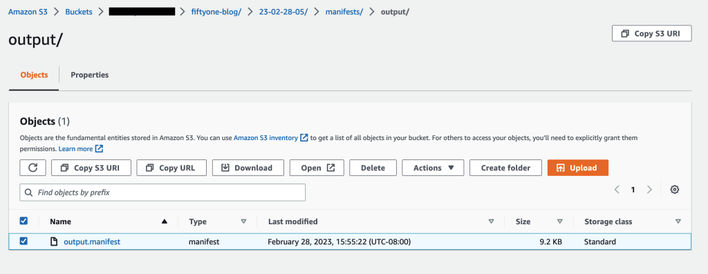
Read the output manifest file:

with open('<path-to-your-output.manifest>', 'r') as fh:
    adjustment_manifest_lines = fh.readlines()

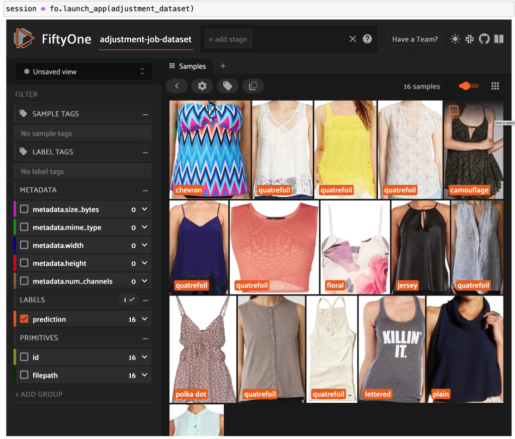
Create a FiftyOne dataset and convert the manifest lines to samples in the dataset:

def get_classification_labels(manifest_line, dataset, attr_name) -> fo.Classifications:
    label_attribute_data = manifest_line.get(attr_name)
    metadata = manifest_line.get(f"{attr_name}-metadata")
 
    annotations = label_attribute_data.get("annotations")
 
    image_data = label_attribute_data.get("image_size")[0]
    width = image_data.get("width")
    height = image_data.get("height")

    predictions = []
    for i, annotation in enumerate(annotations):
        label = metadata.get("class-map").get(str(annotation.get("class_id")))

        confidence = metadata.get("objects")[i].get("confidence")
        
        prediction = fo.Classification(label=label, confidence=confidence)

        predictions.append(prediction)

    return fo.Classifications(classifications=predictions)

def get_bounding_box_labels(manifest_line, dataset, attr_name) -> fo.Detections:
    label_attribute_data = manifest_line.get(attr_name)
    metadata = manifest_line.get(f"{attr_name}-metadata")
 
    annotations = label_attribute_data.get("annotations")
 
    image_data = label_attribute_data.get("image_size")[0]
    width = image_data.get("width")
    height = image_data.get("height")

    detections = []
    for i, annotation in enumerate(annotations):
        label = metadata.get("class-map").get(str(annotation.get("class_id")))

        confidence = metadata.get("objects")[i].get("confidence")

        # Bounding box coordinates should be relative values
        # in [0, 1] in the following format:
        # [top-left-x, top-left-y, width, height]
        bounding_box = [
            annotation.get("left") / width,
            annotation.get("top") / height,
            annotation.get("width") / width,
            annotation.get("height") / height,
        ]

        detection = fo.Detection(
            label=label, bounding_box=bounding_box, confidence=confidence
        )
        
        detections.append(detection)

    return fo.Detections(detections=detections)
    
def get_sample_from_manifest_line(manifest_line, dataset, attr_name):
    """
    For each line in manifest, transform annotations into Fiftyone format
    Args:
        line: manifest line
    Output:
        Fiftyone image sample
    """
    file_name = manifest_line.get("source-ref")[5:].split("/")[-1]
    file_loc = f'200kFashionDatasetExportResult-16Images/data/{file_name}'

    sample = fo.Sample(filepath=file_loc)

    sample['ground_truth'] = get_bounding_box_labels(
        manifest_line=manifest_line, dataset=dataset, attr_name=attr_name
    )
    sample["prediction"] = get_classification_labels(
        manifest_line=manifest_line, dataset=dataset, attr_name=attr_name
    )

    return sample

adjustment_dataset = fo.Dataset("adjustment-job-dataset")

samples = [
            get_sample_from_manifest_line(
                manifest_line=json.loads(manifest_line), dataset=adjustment_dataset, attr_name='smgt-fiftyone-style-adjustment-job'
            )
            for manifest_line in adjustment_manifest_lines
        ]

adjustment_dataset.add_samples(samples)

session = fo.launch_app(adjustment_dataset)

You can now see high-quality labeled data from Ground Truth in FiftyOne.

Conclusion

In this post, we showed how to build high-quality datasets by combining the power of FiftyOne by Voxel51, an open-source toolkit that allows you to manage, track, visualize, and curate your dataset, and Ground Truth, a data labeling service that allows you to efficiently and accurately label the datasets required for training ML systems by providing access to multiple built-in task templates and access to a diverse workforce through Mechanical Turk, third-party vendors, or your own private workforce.

We encourage you to try out this new functionality by installing a FiftyOne instance and using the Ground Truth console to get started. To learn more about Ground Truth, refer to Label Data, Amazon SageMaker Data Labeling FAQs, and the AWS Machine Learning Blog.

Connect with the Machine Learning & AI community if you have any questions or feedback!

Join the FiftyOne community!

Join the thousands of engineers and data scientists already using FiftyOne to solve some of the most challenging problems in computer vision today!

• 200K+ monthly active users
• 1,400+ FiftyOne Slack members
• 2,700+ stars on GitHub
• 3,400+ Meetup members

About the Authors

Shalendra Chhabra is currently Head of Product Management for Amazon SageMaker Human-in-the-Loop (HIL) Services. Previously, Shalendra incubated and led Language and Conversational Intelligence for Microsoft Teams Meetings, was EIR at Amazon Alexa Techstars Startup Accelerator, VP of Product and Marketing at Discuss.io, Head of Product and Marketing at Clipboard (acquired by Salesforce), and Lead Product Manager at Swype (acquired by Nuance). In total, Shalendra has helped build, ship, and market products that have touched more than a billion lives.

Jacob Marks is a Machine Learning Engineer and Developer Evangelist at Voxel51, where he helps bring transparency and clarity to the world’s data. Prior to joining Voxel51, Jacob founded a startup to help emerging musicians connect and share creative content with fans. Before that, he worked at Google X, Samsung Research, and Wolfram Research. In a past life, Jacob was a theoretical physicist, completing his PhD at Stanford, where he investigated quantum phases of matter. In his free time, Jacob enjoys climbing, running, and reading science fiction novels.

Jason Corso is co-founder and CEO of Voxel51, where he steers strategy to help bring transparency and clarity to the world’s data through state-of-the-art flexible software. He is also a Professor of Robotics, Electrical Engineering, and Computer Science at the University of Michigan, where he focuses on cutting-edge problems at the intersection of computer vision, natural language, and physical platforms. In his free time, Jason enjoys spending time with his family, reading, being in nature, playing board games, and all sorts of creative activities.

Brian Moore is co-founder and CTO of Voxel51, where he leads technical strategy and vision. He holds a PhD in Electrical Engineering from the University of Michigan, where his research was focused on efficient algorithms for large-scale machine learning problems, with a particular emphasis on computer vision applications. In his free time, he enjoys badminton, golf, hiking, and playing with his twin Yorkshire Terriers.

Zhuling Bai is a Software Development Engineer at Amazon Web Services. She works on developing large-scale distributed systems to solve machine learning problems.

Read More