In machine learning (ML), data quality has direct impact on model quality. This is why data scientists and data engineers spend significant amount of time perfecting training datasets. Nevertheless, no dataset is perfect—there are trade-offs to the preprocessing techniques such as oversampling, normalization, and imputation. Also, mistakes and errors could creep in at various stages of data analytics pipeline.
In this post, you will learn how to use built-in analysis types in Amazon SageMaker Data Wrangler to help you detect the three most common data quality issues: multicollinearity, target leakage, and feature correlation.
Data Wrangler is a feature of Amazon SageMaker Studio which provides an end-to-end solution for importing, preparing, transforming, featurizing, and analyzing data. The transformation recipes created by Data Wrangler can integrate easily into your ML workflows and help streamline data preprocessing as well as feature engineering using little to no coding. You can also add your own Python scripts and transformations to customize the recipes.
Solution overview
To demonstrate Data Wrangler’s functionality in this post we are going to use the popular Titanic dataset. The dataset describes the survival status of individual passengers on the Titanic and has 14 columns, including the target column. These features include pclass, name, survived, age, embarked, home. dest, room, ticket, boat, and sex. The column pclass refers to passenger class (1st, 2nd, 3rd), and is a proxy for socio-economic class. The column survived is the target column.
Prerequisites
To use Data Wrangler, you need an active Studio instance. To learn how to launch a new instance, see Onboard to Amazon SageMaker Domain.
Before you get started, download the Titanic dataset to an Amazon Simple Storage Service (Amazon S3) bucket.
Create a data flow
To access Data Wrangler in Studio, complete the following steps:
- Next to the user you want to use to launch Studio, choose Open Studio.
- When Studio opens, choose the plus sign on the New data flow card under ML tasks and components.
This creates a new directory in Studio with a .flow file inside, which contains your data flow. The .flow file automatically opens in Studio.

You can also create a new flow by choosing File, then New, and choosing Data Wrangler Flow.

- Optionally, rename the new directory and the
.flowfile.
When you create a new .flow file in Studio, you might see a carousel that introduces you to Data Wrangler. This may take a few minutes.
When the Data Wrangler instance is active, you can see the data flow screen as shown in the following screenshot.
- Choose Use sample dataset to load the titanic dataset.

Create a Quick Model analysis
There are two ways to get a sense for a new (previously unseen) dataset. One is to run Data Quality and Insights Report. This report will provide high level statistics – number features, rows, missing values, etc and surface high priority warnings (if present) – duplicate rows, target leakage, anomalous samples, etc.
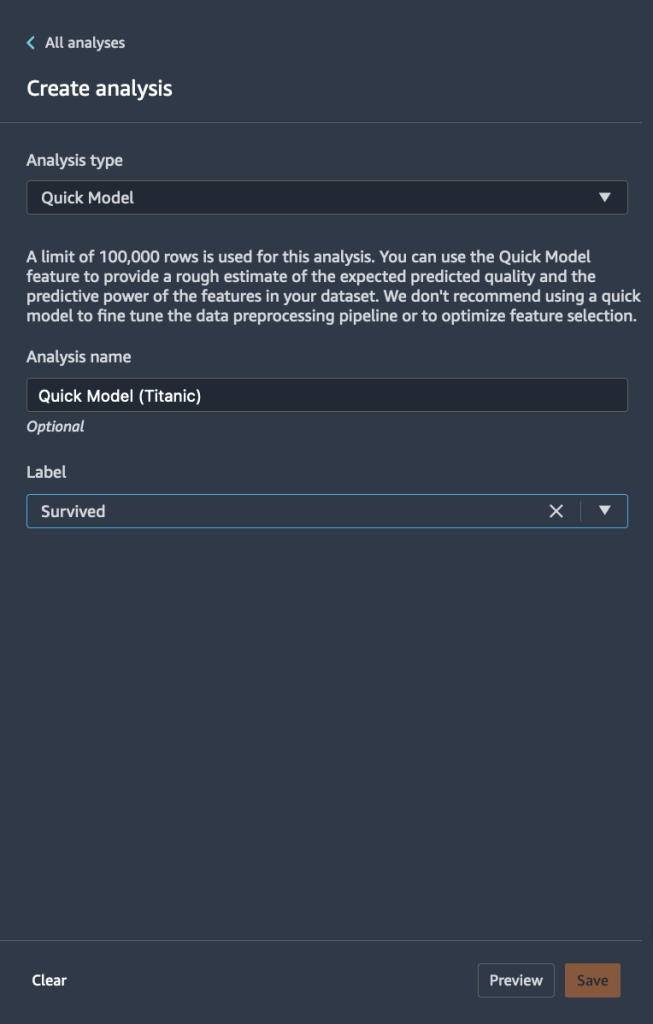
Another way is to run Quick Model analysis directly. Complete the following steps:
- Choose the plus sign and choose Add analysis.

- For Analysis type, choose Quick Model.
- For Analysis name¸ enter a name.
- For Label, choose the target label from the list of your feature columns (
Survived). - Choose Save.
The following graph visualizes our findings.
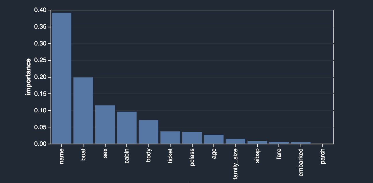
Quick Model trains a random forest with 10 trees on 730 observations and measures prediction quality on the remaining 315 observations. The dataset is automatically sampled and split into training and validation tests (70:30). In this example, you can see that the model achieved an F1 score of 0.777 on the test set. This could be an indicator that the data you’re exploring has the potential of being predictive.
At the same time, a few things stand out right away. The columns name and boat are the highest contributing signals towards your prediction. String columns like name can be both useful and not useful depending on the comprehensive information they carry about the person, like first, middle, and last names alongside the historical time periods and trends they belong to. This column can either be excluded or retained depending on the outcome of the contribution. In this case, a simple preview reveals that passenger names also include their titles (Mr, Dr, etc) which could potentially carry valuable information; therefore, we’re going to keep it. However, we do want to take a closer look at the boat column, which also seems to have a strong predictive power.
Target leakage
First, let’s start with the concept of leakage. Leakage can occur during different stages of the ML lifecycle. Using features that are available only during training but not during inference can also be defined as target leakage. For example, a deployed airbag is not a good predictor for a car crash, because in real life it occurs after the fact.
One of the techniques for identifying target leakage relies on computing ROC values for each feature. The closer the value is to a 1, the more likely the feature is very predictive of the target and therefore the more likely it’s a leaked target. On the other hand, the closer the value is to 0.5 and below (rarely), the less likely this feature contributes anything towards prediction. Finally, values that are above 0.5 and below 1 indicate that the feature doesn’t carry predictive power by itself, but may be a contributor in a group—which is what we’d like to see ideally.
Let’s create a target leakage analysis on your dataset. This analysis together with a set of advanced analyses are offered as built-in analysis types in Data Wrangler. To create the analysis, choose Add Analysis and choose Target Leakage. This is similar to how you previously created a Quick Model analysis.
As you can see in the following figure, your most predictive feature boat is quite close in ROC value to 1, which makes it a possible suspect for target leakage.
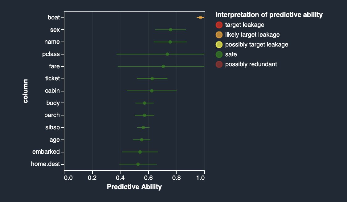
If you read the description of the dataset, the boat column contains the lifeboat number in which the passenger managed to escape. Naturally, there is quite a close correlation with the survival label. The lifeboat number is known only after the fact—when the lifeboat was picked up and the survivors on it were identified. This is very similar to the airbag example. Therefore, the boat column is indeed a target leakage.
You can eliminate it from your dataset by applying the drop column transform in the Data Wrangler UI (choose Handle Columns, choose Drop, and indicate boat). Now if you rerun the analysis, you get the following.

Multicollinearity
Multicollinearity occurs when two or more features in a dataset are highly correlated with one another. Detecting the presence of multicollinearity in a dataset is important because multicollinearity can reduce predictive capabilities of an ML model. Multicollinearity can either already be present in raw data received from an upstream system, or it can be inadvertently introduced during feature engineering. For instance, the Titanic dataset contains two columns indicating the number of family members each passenger traveled with: number of siblings (sibsp) and number of parents (parch). Let’s say that somewhere in your feature engineering pipeline, you decided that it would make sense to introduce a simpler measure of each passenger’s family size by combining the two.
A very simple transformation step can help us achieve that, as shown in the following screenshot.
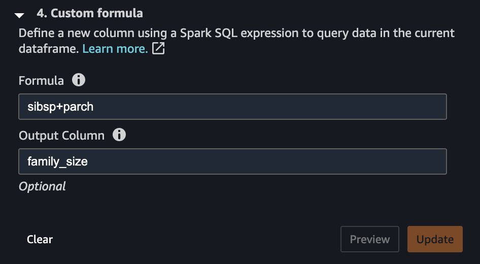
As a result, you now have a column called family_size, which reflects just that. If you didn’t drop the original two columns, you now have very strong correlation between both siblings as well as the parents columns and the family size. By creating another analysis and choosing Multicollinearity, you can now see the following.
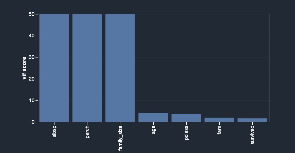
In this case, you’re using the Variance Inflation Factor (VIF) approach to identify highly correlated features. VIF scores are calculated by solving a regression problem to predict one variable given the rest, and they can range between 1 and infinity. The higher the value is, the more dependent a feature is. Data Wrangler’s implementation of VIF analysis caps the scores at 50 and in general, a score of 5 means the feature is moderately correlated, whereas anything above 5 is considered highly correlated.
Your newly engineered feature is highly dependent on the original columns, which you can now simply drop by using another transformation by choosing Manage Columns, Drop Column.
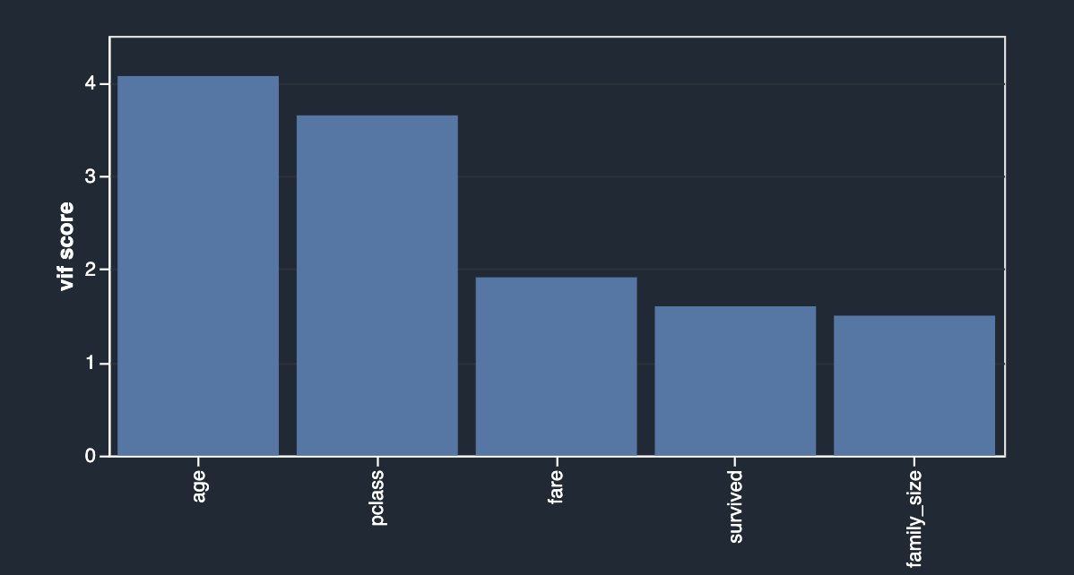
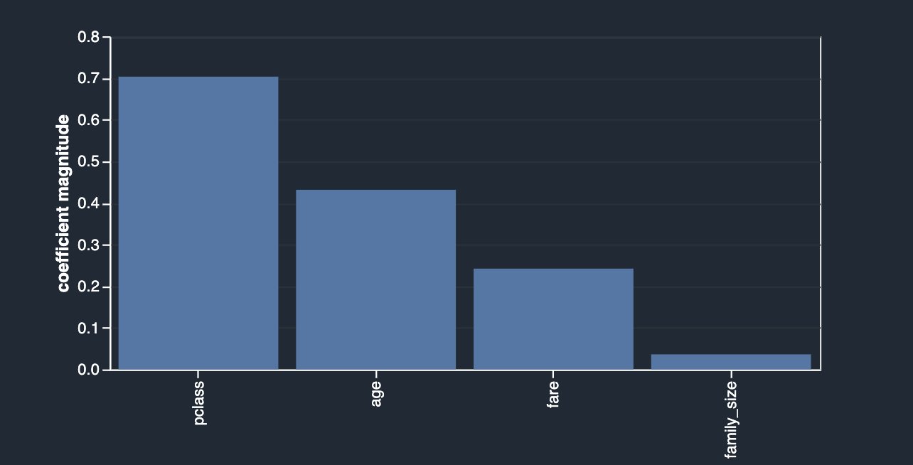
An alternative approach to identify features that have less or more predictive power is to use the Lasso feature selection type of the multicollinearity analysis (for Problem type, choose Classification and for Label column, choose survived).
As outlined in the description, this analysis builds a linear classifier that provides a coefficient for each feature. The absolute value of this coefficient can also be interpreted as the importance score for the feature. As you can observe in your case, family_size carries no value in terms of feature importance due to its redundancy, unless you drop the original columns.
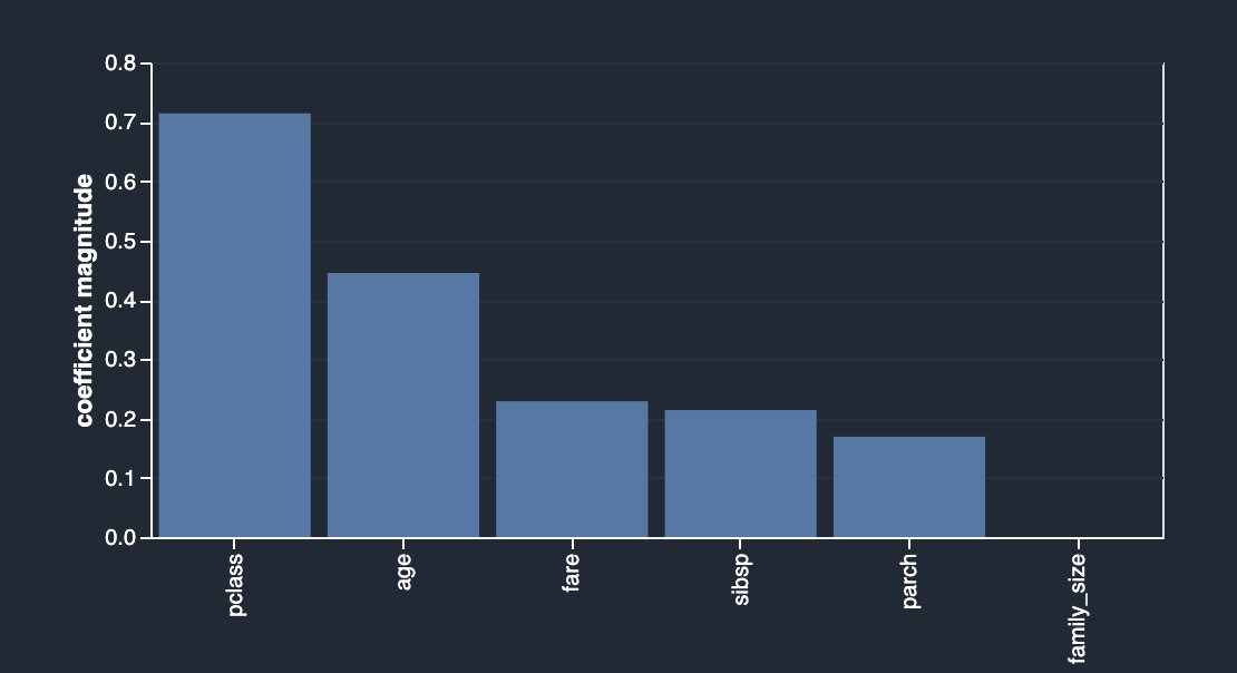
After dropping sibsp and parch, you get the following.
Data Wrangler also provides a third option to detect multicollinearity in your dataset facilitated via Principal Component Analysis (PCA). PCA measures the variance of the data along different directions in the feature space. The ordered list of variances, also known as the singular values, can inform about multicollinearity in your data. This list contains non-negative numbers. When the numbers are roughly uniform, the data has very few multicollinearities. However, when the opposite is true, the magnitude of the top values will dominate the rest. To avoid issues related to different scales, the individual features are standardized to have mean 0 and standard deviation 1 before applying PCA.
Before dropping the original columns (sibsp and parch), your PCA analysis is shown as follows.
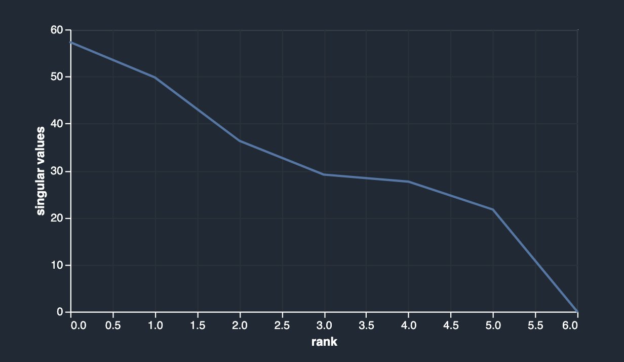
After dropping sibsp and parch, you have the following.
Feature correlation
Correlation is a measure of the degree of dependence between variables. Correlated features in general don’t improve models but can have an impact on models. There are two types of correlation detection features available in Data Wrangler: linear and non-linear.
Linear feature correlation is based on Pearson’s correlation. Numeric-to-numeric correlation is in the range [-1, 1] where 0 implies no correlation, 1 implies perfect correlation, and -1 implies perfect inverse correlation. Numeric-to-categorical and categorical-to-categorical correlations are in the range [0, 1] where 0 implies no correlation and 1 implies perfect correlation. Features that are not either numeric or categorical are ignored.
The following correlation matrix and score table validate and reinforce your previous findings.
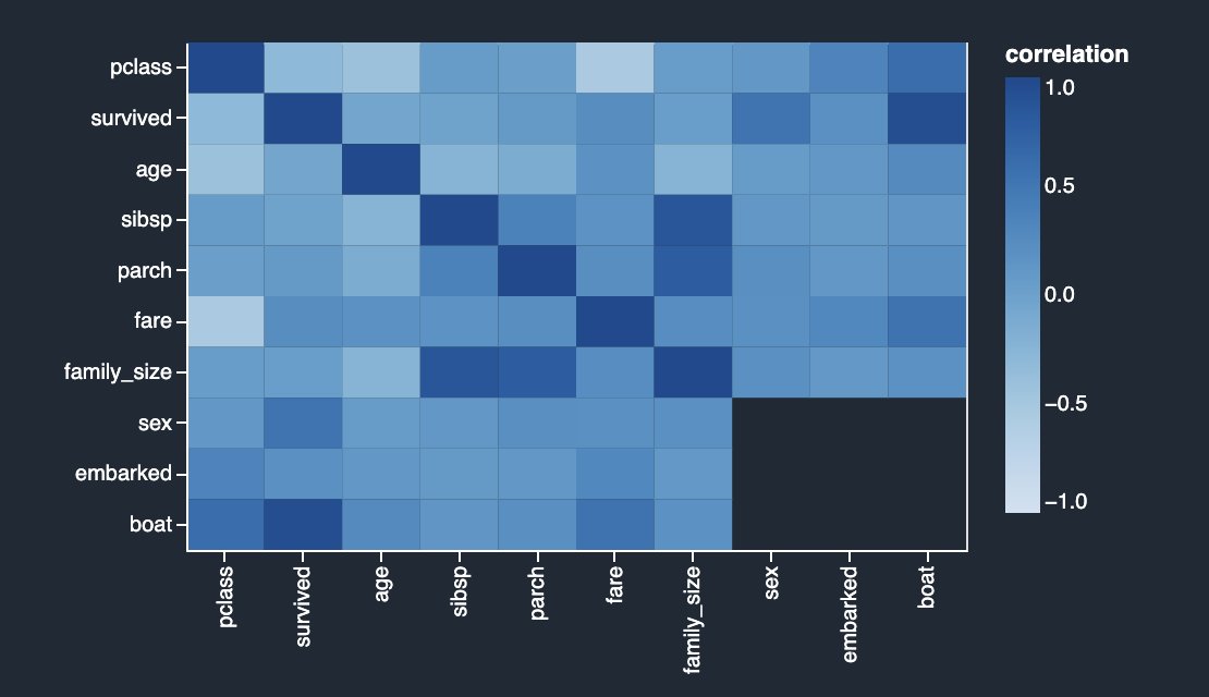

The columns survived and boat are highly correlating with each other. For this example, survived is the target column or the label you’re trying to predict. You saw this previously in your target leakage analysis. On the other hand, columns sibsp and parch are highly correlating with the derived feature family_size. This was confirmed in your previous multicollinearity analysis. We don’t see any strong inverse linear correlation in the dataset.
When two variable changes in a constant proportion, it’s called a linear correlation, whereas when the two variables don’t change in any constant proportion, the relationship is non-linear. Correlation is perfectly positive when proportional change in two variables is in the same direction. In contrast, correlation is perfectly negative when proportional change in two variables is in the opposite direction.
The difference between feature correlation and multi-collinearity (discussed previously) is as follows: feature correlation refers to the linear or non-linear relationship between two variables. With this context, you can define collinearity as a problem where two or more independent variables (predictors) have a strong linear or non-linear relationship. Multicollinearity is a special case of collinearity where a strong linear relationship exists between three or more independent variables even if no pair of variables has a high correlation.
Non-linear feature correlation is based on Spearman’s rank correlation. Numeric-to-categorical correlation is calculated by encoding the categorical features as the floating-point numbers that best predict the numeric feature before calculating Spearman’s rank correlation. Categorical-to-categorical correlation is based on the normalized Cramer’s V test.
Numeric-to-numeric correlation is in the range [-1, 1] where 0 implies no correlation, 1 implies perfect correlation, and -1 implies perfect inverse correlation. Numeric-to-categorical and categorical-to-categorical correlations are in the range [0, 1] where 0 implies no correlation and 1 implies perfect correlation. Features that aren’t numeric or categorical are ignored.
The following table lists for each feature what is the most correlated feature to it. It displays a correlation matrix for a dataset with up to 20 columns.
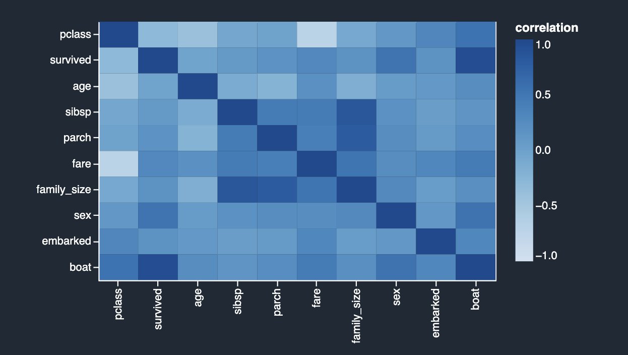
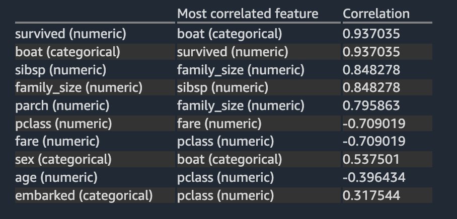
The results are very similar to what you saw in the previous linear correlation analysis, except you can also see a strong negative non-linear correlation between the pclass and fare numeric columns.
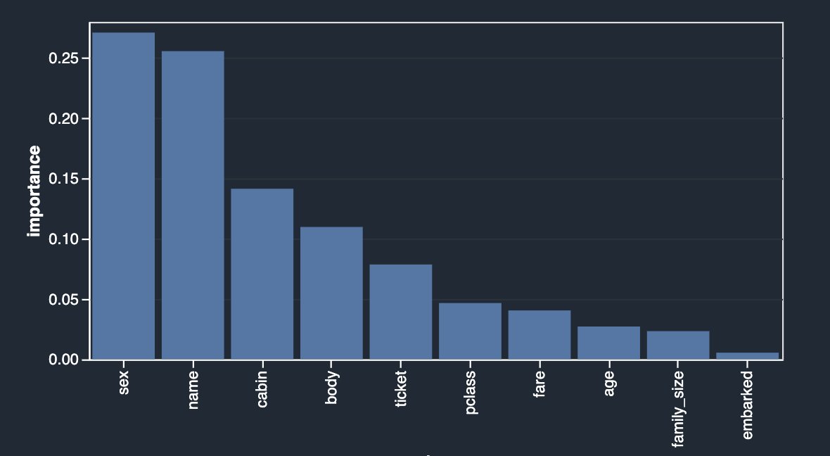
Finally, now that you have identified potential target leakage and eliminated features based on your analyses, let’s rerun the Quick Model analysis to look at the feature importance breakdown again.
The results look quite different than what you started with initially. Therefore, Data Wrangler makes it easy to run advanced ML-specific analysis with a few clicks and derive insights about the relationship between your independent variables (features) among themselves and also with the target variable. It also provides you with the Quick Model analysis type that lets you validate the current state of features by training a quick model and testing how predictive the model is.
Ideally, as a data scientist, you should start with some of the analyses showcased in this post and derive insights into what features are good to retain vs. what to drop.
Summary
In this post, you learned how to use Data Wrangler for exploratory data analysis, focusing on target leakage, feature correlation, and multicollinearity analyses to identify potential issues with training data and mitigate them with the help of built-in transformations. As next steps, we recommend you replicate the example in this post in your Data Wrangler data flow to experience what was discussed here in action.
If you’re new to Data Wrangler or Studio, refer to Get Started with Data Wrangler. If you have any questions related to this post, please add it in the comments section.
About the authors
 Vadim Omeltchenko is a Sr. AI/ML Solutions Architect who is passionate about helping AWS customers innovate in the cloud. His prior IT experience was predominantly on the ground.
 Arunprasath Shankar is a Sr. AI/ML Specialist Solutions Architect with AWS, helping global customers scale their AI solutions effectively and efficiently in the cloud. In his spare time, Arun enjoys watching sci-fi movies and listening to classical music.

