Cutting-edge AI models are becoming extremely large. The cost and overhead of training these models is increasing rapidly, and involves large amounts of engineering and guesswork to find the right training regime. FSDP reduces these costs significantly by enabling you to train much larger models with the same amount of resources. FSDP lowers the memory footprint on your GPUs, and is usable via a lightweight configuration that requires substantially less effort, typically with just a few lines of code.
The main performance gains in FSDP come from maximizing the overlap between network communication and model computation, and eliminating the memory redundancy inherent in traditional data parallel training (DDP). PyTorch FSDP can train models approximately 4x larger on the same server resources as DDP and 20x larger if we combine activation checkpointing and activation offloading.
Since PyTorch 1.12, FSDP is now in beta status, and has added a number of new features that can be tuned to further accelerate your model training.
In this series of blog posts, we will explain multiple performance optimizations you can run with FSDP to boost your distributed training speed and model sizes within the context of your available server resources. We use the HuggingFace T5 3B, 11B and DeepVit, in fine-tuning mode, as the running examples throughout the series.
As a preview of some of the optimizations discussed in this series, we show the before and after performance scaled in Flops below (Note that these results can vary based on your server resources and model architecture).
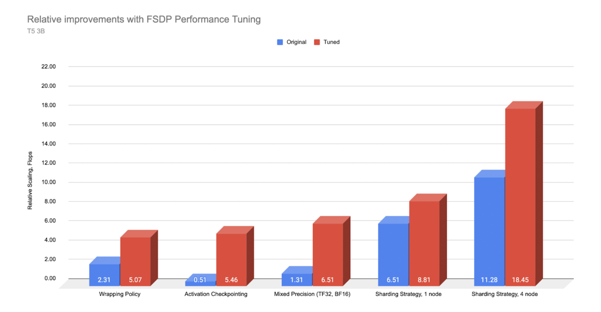
*T5 3B Performance measured on AWS A100 and A10 servers. Original with no optimizations and Tuned with the applied optimization
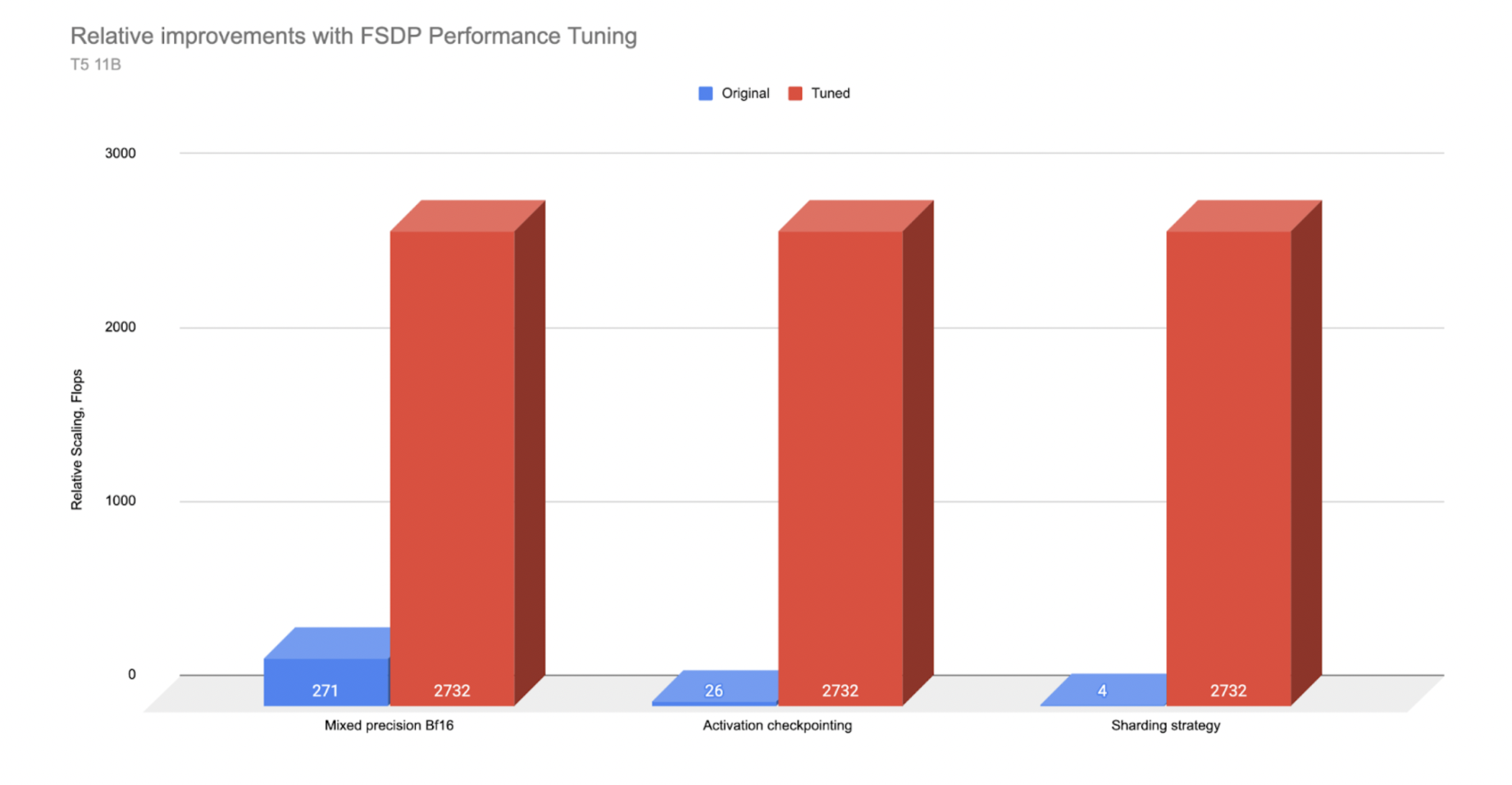
*T5 11B Performance measured on A100 servers. Original with no optimizations and Tuned with the applied optimization
In this first post, we will provide a quick overview of FSDP and how it can make training large- scale AI models more efficient. We will highlight briefly the multiple performance options available, and dive deeper into the details on these in upcoming posts. We will then conclude with an overview on how to leverage AWS parallel cluster for large- scale training with FSDP.
| Optimization | T5 Model | Throughput Improvement |
| Mixed Precision | 3 B | 5x |
| 11 B | 10x | |
| Activation Checkpointing (AC) | 3 B | 10x |
| 11 B | 100x | |
| Transformer Wrapping Policy | 3 B | 2x |
| 11 B | Unable to run the experiment without the Transformer wrapping policy. | |
| Full Shard Strategy | 3 B | 1.5x |
| 11 B | Not able to run with Zero2 |
Performance optimization gains on T5 models over non-optimized.
In our experiments with the T5 3B model, using the transformer wrapping policy resulted in >2x higher throughput measured in TFLOPS versus the default wrapping policy. Activation checkpointing resulted in 10x improvement by reinvesting the freed memory from the checkpoints into larger batch size. Mixed precision with BFloat16 resulted in ~5x improvement versus FP32 and finally the full sharding strategy versus zero2 (DDP) resulted in 1.5x improvement.
We ran similar experiments for a larger model, T5 11B, but the larger model size resulted in some changes to the experiment space. Specifically, we found that two optimizations, transformer wrapping policy and activation checkpointing, were needed to enable us to run these experiments on 3 nodes (each node had 8 A100 gpus with 80 GB of memory). With these optimizations, we could fit a batch size of 50 and get higher throughput compared to removing each one of them. Thus rather than running on/off solely for a single optimization test as with the 3B model, the larger model experiments were done with 1 of 3 optimizations turned on/off while always running the other two in order to allow a usable batch size for both test states for each item.
Based on TFLOP comparisons, with the 11B model, we saw even more payoff from the optimizations. Mixed precision(~10x improvement) and activation checkpointing (~100x improvement) had a much larger impact with the 11B model compared to the 3B parameter model. With mixed precision we could fit ~2x larger batch sizes and with activation checkpointing >15x batch sizes (from 3 with no activation checkpointing to 50 with activation checkpointing) which translated into large throughput improvements.
We also have observed that for these larger models > 3B, using Zero2 sharding strategy would result in minimal room left in memory for the batch data, and had to go with very small batch sizes (e.g 1-2) that essentially makes full sharding strategy a necessity to enable fitting larger batches sizes.
Note – this tutorial assumes a basic understanding of FSDP. To learn more about basics of FSDP please refer to the getting started and advanced FSDP tutorials.
What is FSDP? How does it make Large-Scale Training More Efficient
FSDP expands upon distributed data parallel, by parallelizing not just data, but the model parameters, the optimizer states and gradients associated with the model. Specifically – each GPU only stores a subset of the entire model and the associated subset of optimizer states and gradients.
To show the evolution of distributed training, we can start from the beginning, where AI models were simply trained on a single GPU.
DDP (Distributed Data Parallel) was the initial step up from training with only a single GPU, and was an effort to address the data and model size growth, where multiple GPUs each housed their own copy of the same model. The gain here is that the data for each batch could be split and processed independently on each GPU, all at the same time,thus parallelizing the processing of the data set and increasing training speed by the increasing number of GPUs. The tradeoff is the need to communicate the gradients between each GPU to synchronize the models after the backward pass.
FSDP expands on scaling models by removing the redundancy of optimizer calculations and state storage, as well as gradient and memory storage of model parameters that are present in DDP (DDP = Distributed Data Parallel). This redundancy reduction, along with increased communication overlap where model parameter communication takes place at the same time as model computation, is what allows FSDP to train much larger models with the same resources as DDP.
A key point is that this efficiency also allows for AI models that are larger than a single GPU to be trained. The model size available for training is now increased to the aggregate memory of all GPUs, rather than the size of a single GPU. (And as a point of note, FSDP can go beyond aggregated GPU memory by leveraging CPU memory as well, though we will not directly cover this aspect here).
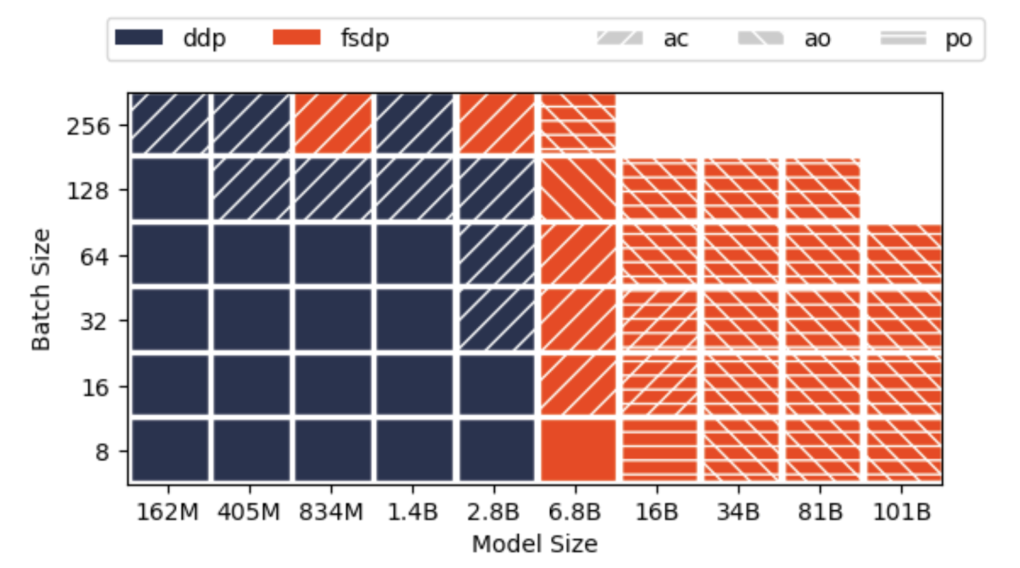
As discussed in a previous blog post, with DDP the largest model that we could train on 32, A100 gpus with 40 GB memory (4 nodes) was up to 3B parameters, and batch size of 128, with the help of activation checkpointing. By contrast, using FSDP we were able to train up to 81B model size, combining activation checkpointing, along with activation and parameter offloading. In another experiment, we benchmarked a 1T parameter model with FSDP using 512 gpus.
For intuition on the parameter level workings of FSDP, below we show an animation detailing how the model parameters are sharded and communicated assuming a two GPU scenario and a simple 8 parameter model:
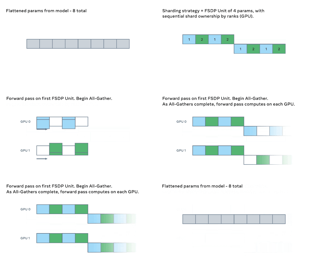
Above – the animations walk through the steps involved with the initial sharding of the model amongst ranks, and we start the all_gathers and forward pass

We continue through the model with the forward pass. After each FSDP unit completes, non-locally owned params are dropped to free memory, and optionally activations can be checkpointed. This continues until we finish the forward pass and compute the loss.
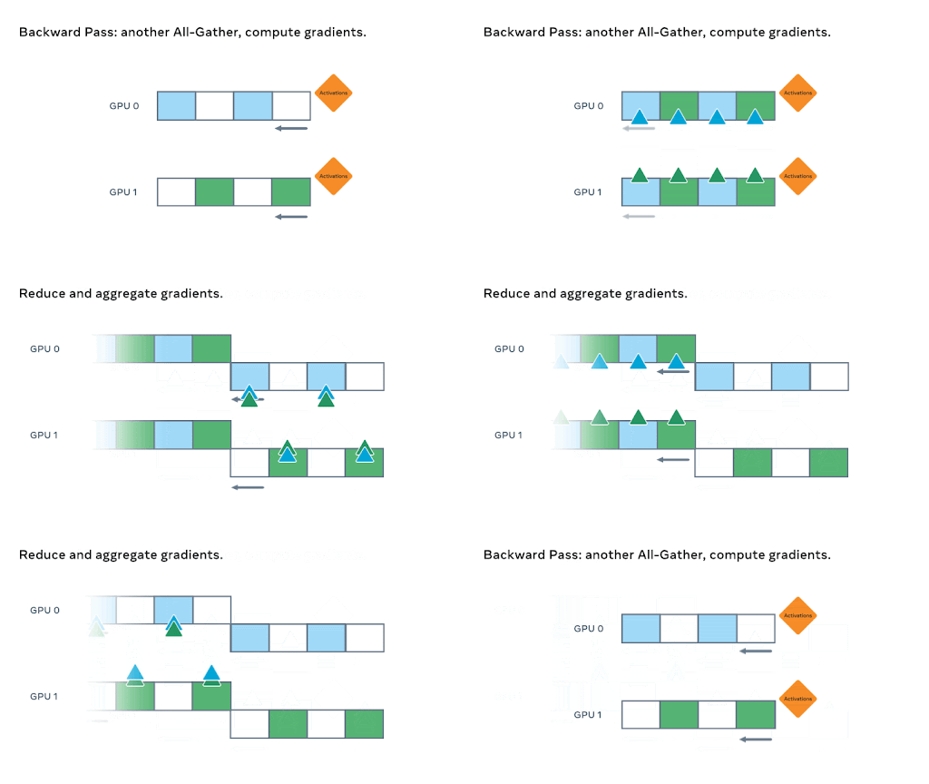
During the backward pass, another all_gather is used to load the parameters and the gradients are computed. These gradients are then reduce_scattered so that the local owners of each param can aggregate and prepare to update the weights.
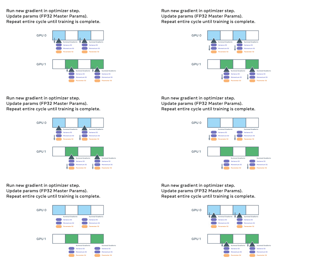
Finally, each rank passes the summed gradients through the optimizer states and updates the weights to complete the mini-batch.
With the model now distributed across the entire set of available GPUs, the logical question is how data moves through the model given this sharding of model parameters.
This is accomplished by FSDP coordinating with all GPUs to effectively share (communicate) the respective parts of the model. The model is decomposed into FSDP units and parameters within each unit are flattened and then sharded across all GPUs. Within each FSDP unit, GPU’s are assigned interleaving ownership of individual model parameters.
By interleaving, we mean the following – assuming 2 gpus with an id of 1 and 2, the FSDP unit ownership pattern would be [12121212], rather than a contiguous chunk of [111222].
During training, an all_gather is initiated and the locally owned model parameters within a FSDP unit are shared by the owner GPU with the other non-owners, when they need it, on a ‘just in time’ type basis. FSDP prefetches parameters to overlap all_gather communication with computation.
When those requested parameters arrive, the GPU uses the delivered parameters, in combination with the parameters it already owns, to create a fully populated FSDP unit. Thus there is a moment where each GPU hits peak memory usage while holding a fully populated FSDP unit.
It then processes the data through the FSDP unit, and drops the parameters it received from other GPU’s to free up memory for the next unit…the process continues over and over proceeding through the entire model to complete the forward pass.The process is then repeated (in general) for the backward pass.(note – this is a simplified version for understanding..there is additional complexity but this should help construct a basic mental model of the FSDP process).
This eliminates much of the memory redundancy present in DDP, but imposes the cost of higher amounts of network communication to shuttle these requested parameters back and forth amongst all the GPUs.Overlapping the communication timing with the computation taking place is the basis of many of the performance improvements we’ll discuss in this series. The key gains are frequently based on the fact that communication can often take place at the same time as computation.As you can surmise, having high communication speed is vital for FSDP performance.
How do I optimize my training with FSDP?
There are four main performance improvements we will cover – the transformer wrapper, activation checkpointing, mixed precision, and selecting the proper sharding strategy. The flowchart below will help as a checklist for tuning options that we will discuss in this post.
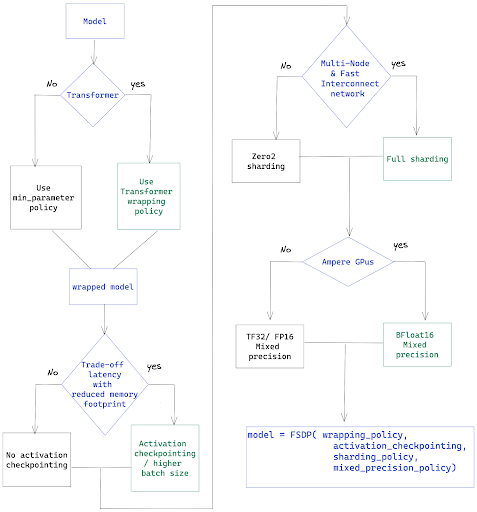
Wrapping policy – for transformers, use Transformer wrapping policy
The first performance optimization is leveraging the FSDP transformer wrapper for transformer models.
One of the pre-defined wrapping policy is size_based_autowrap_policy. With size_based_autowrap_policy, FSDP will traverse the module structure from bottom to top, a new FSDP unit will be created once the current unit has at least the min_num_params specified within the size policy (this defaults to 1e8, or 100M). If the module can not be created as an FSDP unit, FSDP will continue to check its parent module. This size based wrapping policy may not be ideal for some model structures, PyTorch distributed team is actively working on a new default wrapping policy in the next release which is based on size and also module execution order, users can simply tune the size and achieve the optimized performance.
In the current release, you can greatly improve your performance when running Transformer models by using the ‘transformer wrapper’. You will need to provide the appropriate layer class for your model. Here, layer class is the class that houses the Multi-Head Attention and Feed Forward Network.
FSDP will then form the FSDP units around the layer class rather than arbitrary breaks based on parameter size. By sharding the model around layer classes that are uniformly repeated within the transformer, FSDP can create uniform FSDP units that better balance the overlap of computation and communication. By contrast, size based wrapping can produce very uneven or skewed shards for models, which then have uneven matching of compute vs communication overlap. As discussed earlier, the main driver of FSDP high performance is the overlap of communication and computation, and hence why the Transformer wrapper provides improved performance. Note that the Transformer wrapper can also be used for non-transformer models if these models have a list of uniform layers.
Let’s compare the performance difference on a T5, 3B parameter model when running under the default wrapper and the transformer wrapper.
For default wrapping, we don’t need to take any action – we simply pass the model to FSDP as shown:
model = FSDP(
      model,
      device_id=torch.cuda.current_device(),
  )
In this case FSDP will simply wrap the whole model in a single FSDP unit.
Running on an NVIDIA A100-SXM4–40GB with 8 GPUs, we are able to reach 2.3 TFlops and 95% GPU memory utilization with a batch size of 14.
However, since T5 is a transformer model, we are better served to leverage the transformer wrapper for this model.
To use that, we need to isolate the layer class for the transformer, and then pass it in to create our transformer wrapper.
from transformers.models.t5.modeling_t5 import T5Block
And now we can create our Transformer wrapper:
transformer_auto_wrapper_policy = functools.partial(
        transformer_auto_wrap_policy,
        transformer_layer_cls={
            T5Block,  # < ---- Your Transformer layer class
        },
    )
With our model aware wrapper ready, we can initialize FSDP:
# invoke FSDP with your transformer wrapper policy:
model = FSDP(
        model,
        auto_wrap_policy=transformer_auto_wrapper_policy,
        device_id=torch.cuda.current_device(),  # streaming init
    )
Running this wrapped model, we can see some substantial performance gains.We can fit nearly double the batch size, going to 28, and with better memory and communication efficiency, we see a TFlops increase to 5.07 from 2.3.
Thus, we’ve increased our training throughput by over 200% (2.19x) due to providing greater model info to FSDP! The transformer wrapping policy results in more fine-grained and balanced FSDP units each holding a layer class, which leads to a more effective communication-computation overlap.
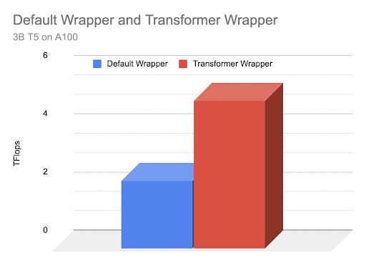
Above: Graphical comparison of TFlops based on wrapper type
If you are training a Transformer model, it pays to configure your training with FSDP using the transformer wrapper. For more information on how to isolate your layer class, please see our in depth video on Transformer wrapping here, where we walk through a number of transformers showing where the layer class can be found.
Mixed precision – use BF16 if you have an Ampere architecture GPU
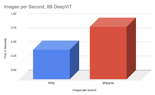
FSDP supports a flexible mixed precision policy that gives you granular control over parameters, gradients and buffer data types. This lets you easily leverage BFloat16 or FP16 to increase your training speed by up to 70%.
*Note that BFloat 16 is only available on Ampere type GPUs. On AWS this is available with p4dn and g5 instances.
By way of comparison, we can show a 77% speed improvement when comparing fully tuned BFloat16 vs FP32 on an 8B DeepVit model.
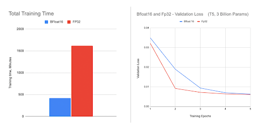
We have obtained even greater acceleration using BFloat16 in fine-tuning a 3B HuggingFace T5 model as shown in the figures below. We observed that because of the lower precision the validation loss of BFloat16 is slightly behind in the first few epochs, but it is able to catch up and results in the same final accuracy as FP32.
To use mixed precision, we create a policy with our desired data types, and pass it in during the FSDP initialization.
To create our policy, we need to import the MixedPrecision class, and then define our custom policy using our customized class:
from torch.distributed.fsdp import MixedPrecision
bfSixteen = MixedPrecision(
   param_dtype=torch.bfloat16,
   # Gradient communication precision.
   reduce_dtype=torch.bfloat16,
   # Buffer precision.
   buffer_dtype=torch.bfloat16,
)
model = FSDP(
       model,
       auto_wrap_policy=transformer_auto_wrapper_policy,
       mixed_precision=bfloatPolicy)
You can mix and match the precision for parameters, gradients and buffers as you prefer:
comboPolicy = MixedPrecision(
        # Param precision
        param_dtype=torch.bfloat16,
        # Gradient communication precision.
        reduce_dtype=torch.float32,
        # Buffer precision.
        buffer_dtype=torch.float32,
    )
For training with FP16, you will need to also use the ShardedGradScaler, which we will cover in subsequent posts. For BFloat16, it is a drop-in replacement.
AnyPrecision Optimizer – going beyond mixed precision with full BF16 training
Mixed precision training, both in FSDP and elsewhere, maintains the working weights in the reduced datatype (BF16 or FP16) while keeping the master weights in full FP32. The reason for the master weights in FP32 is that running in pure BF16 will result in ‘weight stagnation’, where very small weight updates are lost due to the lower precision, and the accuracy flatlines over time while FP32 weights can continue to improve from these small updates.
In order to resolve this dilemma, we can use the new AnyPrecision optimizer available in TorchDistX (Torch Distributed Experimental) that allows you to successfully train and keep the master weights in pure BF16 instead of FP32. In addition, unlike the typical storage of optimizer states in FP32, AnyPrecision is able to maintain states in pure BF16 as well.
AnyPrecision enables pure BF16 training by maintaining an extra buffer that tracks the precision lost during the weight updates and re-applies that during the next update…effectively resolving the weight stagnation issue without requiring FP32.
As a comparison of the throughput gains available with pure BF16 training using AnyPrecision, we ran experiments using FSDP with the T5 11B model with regular FP32 training, Mixed Precision training with BF16, and pure BF16 training using the AnyPrecision optimizer on 3 nodes with A100 gpus as mentioned previously.
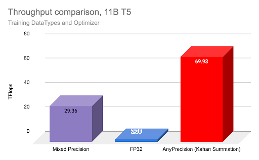
As shown above, training with AnyPrecision and pure BF16 resulted in 2x the throughput vs Mixed Precision, and over 20x improvement vs FP32.
The potential tradeoff is the impact on final accuracy – in the cases we tested, the accuracy was equal or better than FP32 due to a regularization effect from the slightly reduced precision, but your results may vary.
AnyPrecision optimizer is available for you to test with here, and is a drop in replacement for AdamW optimizer.
Activation checkpointing – increasing throughput by trading compute for memory
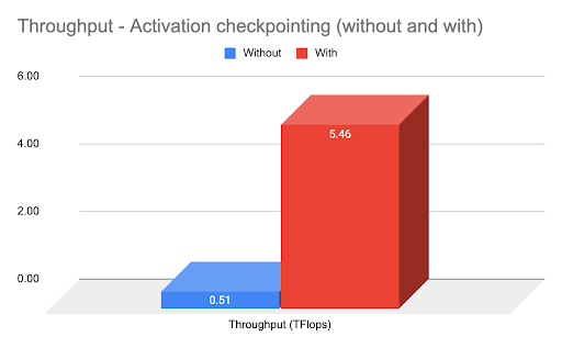
FSDP supports activation checkpointing once the model has been sharded, and makes it easy to implement. The graph above shows ~4x throughput improvement using activation checkpointing.
Activation checkpointing is where the intermediate activations are freed during the forward pass, and a checkpoint is left as a placeholder. This generally increases available GPU memory by over 30%.
The tradeoff is that during the backward pass, these previously removed intermediate activations must be re-calculated again using information in the checkpoint (duplicate compute), but by leveraging the increased GPU memory, one can increase the batch size such that the net throughput can increase substantially.
# verify we have FSDP activation support ready by importing:
from torch.distributed.algorithms._checkpoint.checkpoint_wrapper import (
   checkpoint_wrapper,
   CheckpointImpl,
   apply_activation_checkpointing_wrapper,
)
The steps required to implement activation checkpointing is to first import the FSDP checkpointing functions. We need declare our checkpointer wrapper type which is non-reentrant and create a check function to identify which layer to wrap as follows
non_reentrant_wrapper = partial(
    checkpoint_wrapper,
    offload_to_cpu=False,
    checkpoint_impl=CheckpointImpl.NO_REENTRANT,
)
check_fn = lambda submodule: isinstance(submodule, T5Block)
apply_activation_checkpointing_wrapper(
       model, checkpoint_wrapper_fn=non_reentrant_wrapper, check_fn=check_fn
   )
Important note – this must be run after the model has been initialized with FSDP.
However, hopefully you’ve seen how some initial tuning with FSDP options can have a large impact on your training performance.
With that, we turn our attention from how to scale within FSDP, to how to scale your server hardware for FSDP using AWS.
Large Scale Training with FSDP on AWS – For multi-node prioritize high speed network
AWS provides several services that can be used to run distributed training with FSDP: Amazon EC2 Accelerated Computing instances, AWS ParallelCluster, and Amazon Sagemaker.
In this series of blog posts, we used Amazon EC2 p4d instances in a single-instance multi-GPU configuration and in a multi-instance configuration using AWS ParallelCluster and SageMaker in order to run our training jobs.
Here, we’ll focus specifically on AWS parallel cluster and provide an overview of how to utilize it for training purposes.
AWS ParallelCluster Setup
AWS ParallelCluster is an open source, cluster management tool that makes it easy for you to deploy and manage High Performance Computing (HPC) clusters on AWS. AWS ParallelCluster uses yaml configuration files to provision all the necessary resources. It also supports multiple instance types, job submission queues, shared file systems like Amazon EFS (NFS) or Amazon FSx for Lustre, and job schedulers like AWS Batch and Slurm.
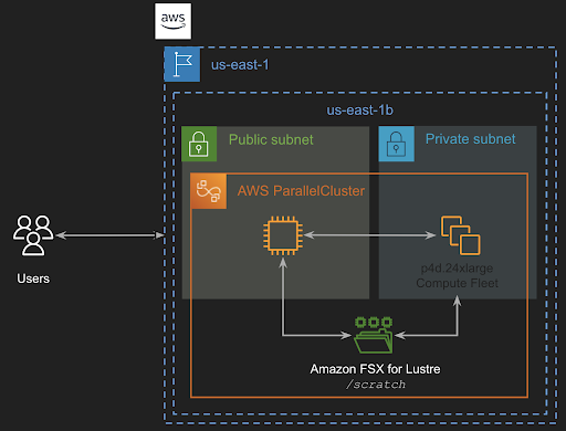
Workflow on Clusters
The high level idea is to have a cluster that has a head node which controls the compute nodes. The actual training job runs on the compute nodes. Overall steps to run a training job on a cluster are as follows:
- Set up an AWS ParallelCuster (we discuss below)
- Connect to the head node, and import the training code/ setup the environment.
- Pull the data and place it in a shared folder that compute nodes can access (FSx Lustre drive).
- Run the training job using a job scheduler (in this case Slurm).
Setup AWS ParallelCuster
To setup AWS ParallelCluster,
-
Deploy a network stack. This step is optional since you could use your account default VPC and let AWS ParallelCluster create your subnets and security groups. However, we prefer to compartmentalize our desired network infrastructure and do this deployment via a CloudFormation stack.
Since we deploy a public and a private subnet, we want to create them into an Availability Zone that contains our target instances, in this case p4d. We consult their availability in the region we use (us-east-1) through the following AWS CLI command:
aws ec2 describe-instance-type-offerings --location-type availability-zone --filters Name=instance-type,Values=p4d.24xlarge --region us-east-1 --output tableWe see three availability zones containing p4d instances, we pick one of them (
us-east-1c, yours may be different) when deploying our network stack. This can be done with the AWS Console or the AWS CLI. In our case we use the latter as followsaws cloudformation create-stack --stack-name VPC-Large-Scale --capabilities CAPABILITY_IAM --template-body file://VPC-Large-Scale.yaml --parameters ParameterKey=SubnetsAZ,ParameterValue=us-east-1cCloudFormation will deploy our new VPC, subnets, security groups and endpoints on our behalf. Once done, you can retrieve the IDs of the public and private subnets by querying the stack outputs and the values
PublicSubnetandPrivateSubnet.For example, using the AWS CLI for the private subnet:
aws cloudformation describe-stacks --stack-name VPC-Large-Scale --query "Stacks[0].Outputs[?OutputKey=='PrivateSubnet'].OutputValue" --output text -
Create ParallelCluster, The cluster configuration file specifies the resources for our cluster. These resources include instance type for Head node, compute nodes, access to S3 buckets, shared storage where our data will be located. We will use Amazon FSx for Lustre that offers a fully managed shared storage service with Lustre.
Here is an example of a cluster configuration file. We can use AWs ParallelCluster CLI to create the cluster. Please note that the private and public subnet IDs will need to be replaced by the ones you retrieved earlier. You will be able to control the cluster using the AWS ParallelCluster CLI to start, stop, pause, etc.
pcluster create-cluster --cluster-name my-hpc-cluster --cluster-configuration cluster.yaml -
SSH to Head node – once the cluster is ready, we can connect to the Head node using the SSH protocol, pull our training code with and place the data in the shared storage specified in the cluster configuration file.
pcluster ssh --cluster-name cluster -i your-key_pair -
Launch the training job – now that we have the data and training code, we can launch the slurm job for training. Here is an example of a slurm script to launch the job using torchrun.
More details on how to set up the cluster is out of the scope of this post, however we will have a separate post on it.
What’s next?
With this post we provided a high level overview of FSDP and how it efficiently scales distributed AI training. The flowchart included will help provide a checklist for you to review tuning options discussed such as the transformer wrapper and activation checkpointing.
In the next posts, we will continue with the T5 model and go deeper into each of the topics above, specifically with sharding strategy and other optimizations to provide more insight and details. For now, a good reference for the sharding strategy is in our video tutorial here:
If you have questions or find an issue, please find the authors Less, Hamid and Geeta or open an issue on PyTorch github.
Special thanks to:
Pytorch Distributed team, Shen Li, Rohan Varma, Yanli Zhao, Andrew Gu, Anjali Sridhar, Ana Simoes, Pierre-Yves Aquilanti, Sundar Ranganathan, and the broader AWS team for supporting us with providing infrastructure and technical support for running the large scale experiments.
Resources:
