Forecasting AWS spend using the AWS Cost and Usage Reports, AWS Glue DataBrew, and Amazon Forecast

AWS Cost Explorer enables you to view and analyze your AWS Cost and Usage Reports (AWS CUR). You can also predict your overall cost associated with AWS services in the future by creating a forecast of AWS Cost Explorer, but you can’t view historical data beyond 12 months. Moreover, running custom machine learning (ML) models on historical data can be labor and knowledge intensive, often requiring some programming language for data transformation and building models.

In this post, we show you how to use Amazon Forecast, a fully managed service that uses ML to deliver highly accurate forecasts, with data collected from AWS CUR. AWS Glue DataBrew is a new visual data preparation tool that makes it easy for data analysts and data scientists to clean and normalize data to prepare it for analytics and ML. We can use DataBrew to transform CUR data into the appropriate dataset format, which Forecast can later ingest to train a predictor and create a forecast. We can transform the data into the required format and predict the cost for a given service or member account ID without writing a single line of code.

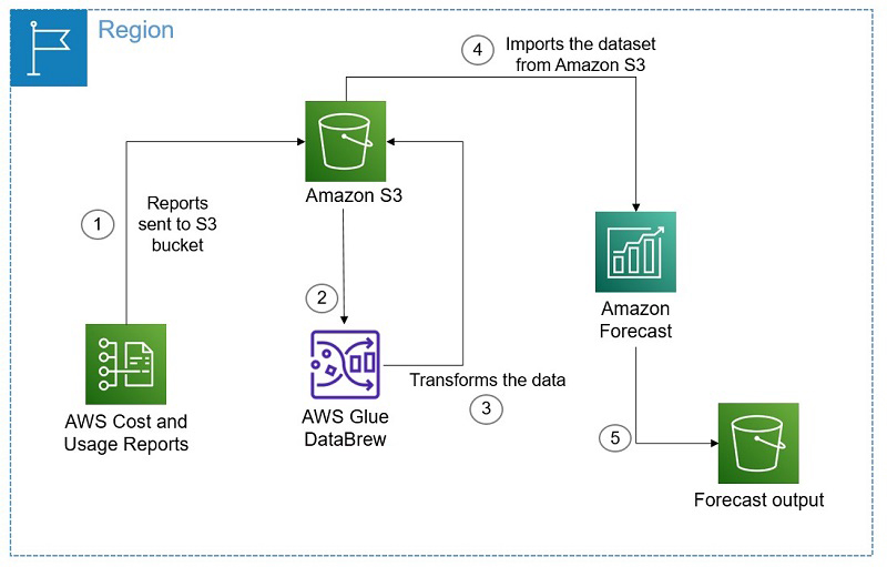
The following is the architecture diagram of the solution.

Walkthrough

You can choose hourly, daily, or monthly reports that break out costs by product or resource (including self-defined tags) using the AWS CUR. AWS delivers the CUR to an Amazon Simple Storage Service (Amazon S3) bucket, where this data is securely retained and accessible. Because cost and usage data are timestamped, you can easily deliver the data to Forecast. In this post, we use CUR data that is collected on a daily basis. After you set up the CUR, you can use DataBrew to transform the CUR data into the appropriate format for Forecast to train a predictor and create a forecast output without writing a single line of code. In this post, we walk you through the following high-level tasks:

1. Prepare the data.
2. Transform the data.
3. Prepare the model.
4. Validate the predictors.
5. Generate a forecast.

Prerequisites

Before we begin, let’s create an S3 bucket to store the results from the DataBrew job. Remember the bucket name, because we refer to this bucket during deployment. With DataBrew, you can determine the transformations and then schedule them to run automatically on new daily, weekly, or monthly data as it comes in without having to repeat the data preparation manually.

Preparing the data

To prepare your data, complete the following steps:

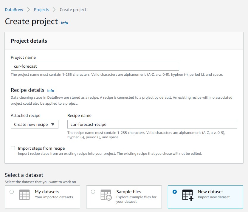
1. On the DataBrew console, create a new project.
2. For Select a dataset, select New dataset.

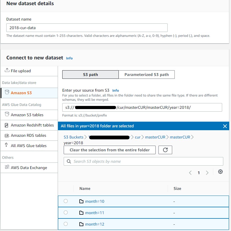
When selecting CUR data, you can select a single object, or the contents of an entire folder.

If you don’t have substantial or interesting usage in your report, you can use a sample file available on Verify Your CUR Files Are Being Delivered. Make sure you follow the folder structure when uploading the Parquet files, and make sure the folder only contains the Parquet files needed. If the folder has other random files, it errors out.

3. Create a role in AWS Identity and Access Management (IAM) that allows DataBrew to access CUR files.

You can either create a custom role or have DataBrew create one on your behalf.

4. Choose Create project.

DataBrew takes you to the the project screen to view and analyze your data.

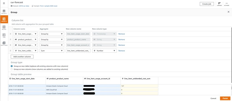
First, we need to select only those columns required for Forecast. We can do this by grouping the columns by our desired dimensions and creating a summed column of unblended costs.

5. Choose the Group icon on the navigation bar and group by the following columns:
   1. line_item_usage_start_date, GROUP BY
   2. product_product_name, GROUP BY
   3. line_item_usage_account_id, GROUP BY
   4. line_item_unblended_cost, SUM

6. For Group type, select Group as new table to replace all existing columns with new columns.

This extracts only the required columns for our forecast.

7. Choose Finish.

In DataBrew, a recipe is a set of data transformation steps. As you progress, DataBrew documents your data transformation steps. You can save and use these recipes in the future for new datasets and transformation iterations.

8. Choose Add step.
9. For Create column options¸ choose Based on functions.
10. For Select a function, choose DATEFORMAT.
11. For Values using, choose Source column.
12. For Source column, choose line_item_usage_start_date.
13. For Date format, choose yyyy-mm-dd.

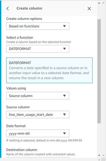
14. Add a destination column of your choice.
15. Choose Apply.

We can delete the original timestamp column because it’s a duplicate.

16. Choose Add step.
17. Delete the original line_item_usage_start_date column.
18. Choose Apply.

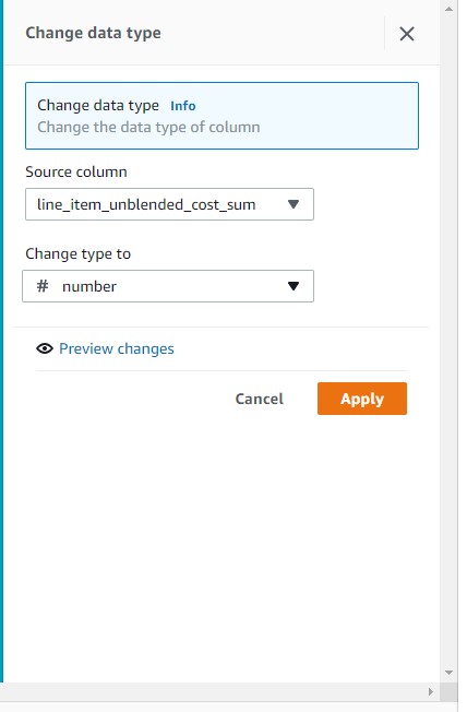
Finally, let’s change our summed cost column to a numeric data type.

19. Choose the Setting icon for the line_item_unblended_cost_sum column.
20. For Change type to, choose # number.
21. Choose Apply.

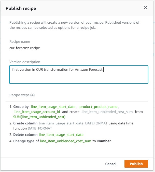
DataBrew documented all four steps of this recipe. You can version recipes as your analytical needs change.

22. Choose Publish to publish an initial version of the recipe.

Transforming the data

Now that we have finished all necessary steps to transform our data, we can instruct DataBrew to run the actual transformation and output the results into an S3 bucket.

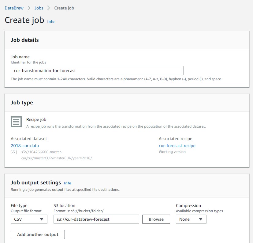
1. On the DataBrew project page, choose Create job.
2. For Job name, enter a name for your job.
3. Under Job output settings¸ for File type¸ choose CSV.
4. For S3 location, enter the S3 bucket we created in the prerequisites.

5. Choose either the IAM role you created or the one DataBrew created for you.
6. Choose Run job.

It may take several minutes for the job to complete. When it’s complete, navigate to the Amazon S3 console and choose the S3 bucket to find the results. The bucket contains multiple CSV files with keys starting with _part0000.csv. As a fully managed service, DataBrew can run jobs in parallel on multiple nodes to process large files on your behalf. This isn’t a problem because you can specify an entire folder for Forecast to process.

Scheduling DataBrew jobs

You can schedule DataBrew jobs to transform the CUR to update to provide Forecast with a refreshed dataset.

1. On the Job menu, choose the Schedules tab.
2. Provide a schedule name.
3. Specify the run frequency on the day and hour.
4. Optionally, provide the start time for the job run.

DataBrew then runs the job per your configuration.

Preparing the model

To prepare your model, complete the following steps:

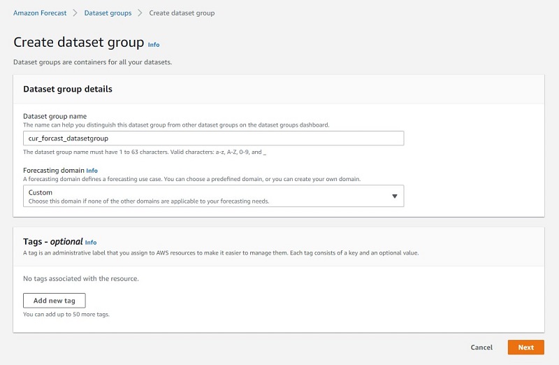
1. On the Forecast console, choose Dataset groups.
2. Choose Create dataset group.
3. For Dataset group name, enter a name.
4. For Forecasting domain, choose Custom.
5. Choose Next.

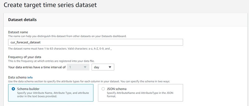
We need to create a target time series dataset.

6. For Frequency of data, choose 1 day.

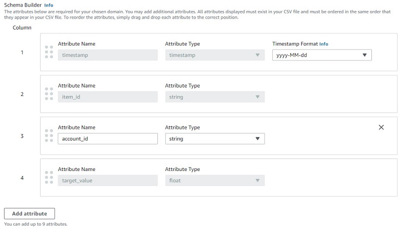
We can define the data schema to help Forecast become aware of our data types.

7. Drag the timestamp attribute name column to the top of the list.
8. For Timestamp Format, choose yyyy-MM-dd. 

This aligns to the data transformation step we completed in DataBrew.

9. Add an attribute as the third column with the name as account_id and attribute type as string.

10. For Dataset import name, enter a name.
11. For Select time zone, choose your time zone.
12. For Data location, enter the path to the files in your S3 bucket.

If you browse Amazon S3 for the data location, you can only choose individual files. Because our DataBrew output consists of multiple files, enter the S3 path to the files’ location and make sure that a slash (/) is at the end of the path.

13. For IAM role, you can create a role so Forecast has permissions to only access the S3 bucket containing the DataBrew output.
14. Choose Start import.

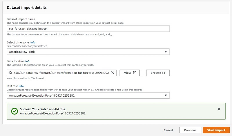
Forecast takes approximately 45 minutes to import your data. You can view the status of your import on the Datasets page.

15. When the latest import status shows as Active, proceed with training a predictor.
16. For Predictor name, enter a name.
17. For Forecast horizon, enter a number that tells Forecast how far into the future to predict your data.

The forecast horizon can’t exceed one-third length of the target time series.

18. For Forecast frequency, leave at 1 day.
19. If you’re unsure of which algorithm to use to train your model, for Algorithm selection, select Automatic (AutoML). 

This option lets Forecast select the optimal algorithm for your datasets, which automatically trains a model and provides accuracy metrics and generate forecasts. Otherwise, you can manually select one of the built-in algorithms. For this post, we use AutoML.

20. For Forecast dimension, choose account_id.

This allows Forecast to predict cost by account ID in addition to product name.

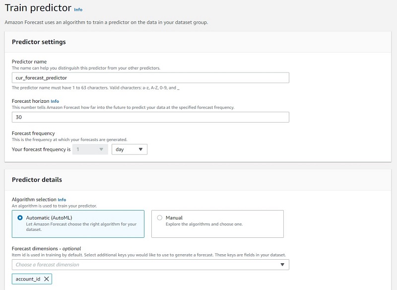
21. Leave all other options at their default and choose Train predictor.

Forecast begins training the optimal ML model on your dataset. This could take up to an hour to complete. You can check on the training status on the Predictors page. You can generate a forecast after the predictor training status shows as Active.

When it’s complete, you can see that Forecast chose DeepAR+ as the optimal ML algorithm. DeepAR+ analyzes the data as similar time series across a set of cross-functional units. These time series groupings demand different product names and account IDs. In this case, it can be beneficial to train a single model jointly over all time series.

Validating the predictors

Forecast provides comprehensive accuracy metrics to help you understand the performance of your forecasting model, and can compare it to the previous forecasting models you’ve created that may have looked at a different set of variables or used a different period of time for the historical data.

By validating our predictors, we can measure the accuracy of forecasts for individual items. In the Algorithm metrics section on the predictor details page, you can view the accuracy metrics of the predictor, which include the following:

• WQL – Weighted quantile loss at a given quantile
• WAPE – Weighted absolute percentage error
• RMSE – Root mean square error

As another method, we can export the accuracy metrics and forecasted values using algorithm metrics for our predictor. With this method, you can view accuracy metrics for specific services when forecasting, such as Amazon Elastic Compute Cloud (Amazon EC2) or Amazon Relational Database Service (Amazon RDS).

1. Select the predictor you created.
2. Choose Export backtest results.
3. For Export name¸ enter a name.
4. For IAM role¸ choose the role you used earlier.
5. For S3 predictor backtest export location, enter the S3 path where you want Forecast to export the accuracy metrics and forecasted values.

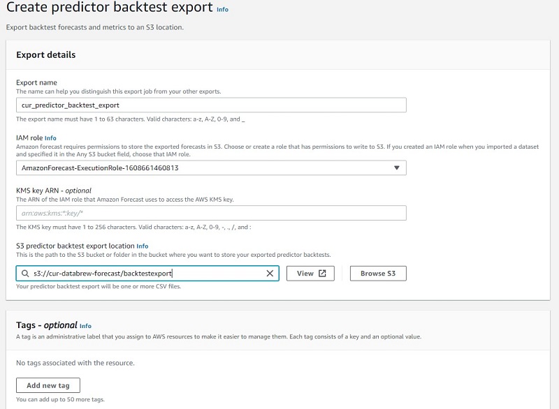
6. Choose Create predictor backtest report.

After some time, Forecast delivers the export results to the S3 location you specified. Forecast exports two files to Amazon S3 in two different folders: forecasted-values and accuracy-metric-values. For more information about accuracy metrics, see Amazon Forecast now supports accuracy measurements for individual items. 

Generating a forecast

To create a forecast, complete the following steps:

1. For Forecast name, enter a name.
2. For Predictor¸ choose the predictor you created.
3. For Forecast types, you can specify up to five quantile values. For this post, we leave it blank to use the defaults.
4. Choose Create new forecast.

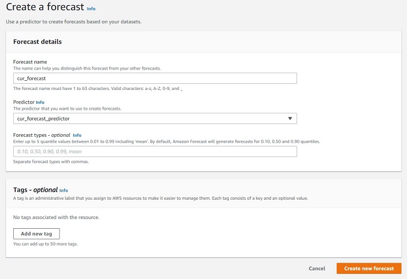
When it’s complete, the forecast status shows as Active. Let’s now create a forecast lookup.

5. For Forecast¸ choose the forecast you just created.
6. Specify the start and end date within the bounds of the forecast.
7. For Value, enter a service name (for this post, Amazon RDS).
8. Choose Get Forecast.

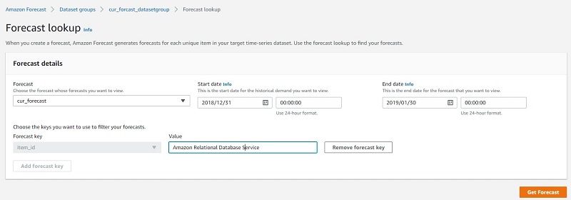
Forecast returns P10, P50, and P90 estimates as the default lower, middle, and upper bounds, respectively. For more information about predictor metrics, see Evaluating Predictor Accuracy. Feel free to explore different forecasts for different services in addition to creating a forecast for account ID.

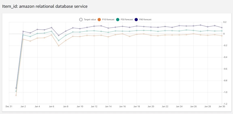
Congratulations! You’ve just created a solution to retrieve forecasts on your CUR by using Amazon S3, DataBrew, and Forecast without writing a single line of code. With these services, you only pay for what you use and don’t have to worry about managing the underlying infrastructure to run transformations and ML inferences. 

Conclusion

In this post, we illustrated how to use DataBrew to transform the CUR into a format for Forecast to make predictions without any need for ML expertise. We created datasets, predictors, and a forecast, and used Forecast to predict costs for specific AWS services. To get started with Amazon Forecast, visit the product page. We also recently announced that CUR is available to member (linked) accounts. Now any entity with the proper permissions under any account within an AWS organization can use the CUR to view and manage costs.

About the Authors

Jyoti Tyagi is a Solutions Architect with great passion for artificial intelligence and machine learning. She helps customers to architect highly secured and well-architected applications on the AWS Cloud with best practices. In her spare time, she enjoys painting and meditation.

Peter Chung is a Solutions Architect for AWS, and is passionate about helping customers uncover insights from their data. He has been building solutions to help organizations make data-driven decisions in both the public and private sectors. Outside of work, he enjoys cooking and spending time with his family.

Read More