GPUs can significantly speed up deep learning training, and have the potential to reduce training time from weeks to just hours. However, to fully benefit from the use of GPUs, you should consider the following aspects:
- Optimizing code to make sure that underlying hardware is fully utilized
- Using the latest high performant libraries and GPU drivers
- Optimizing I/O and network operations to make sure that the data is fed to the GPU at the rate that matches its computations
- Optimizing communication between GPUs during multi-GPU or distributed training
Amazon SageMaker is a fully managed service that enables developers and data scientists to quickly and easily build, train, and deploy machine learning (ML) models at any scale. In this post, we focus on general techniques for improving I/O to optimize GPU performance when training on Amazon SageMaker, regardless of the underlying infrastructure or deep learning framework. You can typically see performance improvements up to 10-fold in overall GPU training by just optimizing I/O processing routines.
The basics
A single GPU can perform tera floating point operations per second (TFLOPS), which allows them to perform operations 10–1,000 times faster than CPUs. For GPUs to perform these operations, the data must be available in the GPU memory. The faster you load data into GPU, the quicker it can perform its operation. The challenge is to optimize I/O or the network operations in such a way that the GPU never has to wait for data to perform its computations.
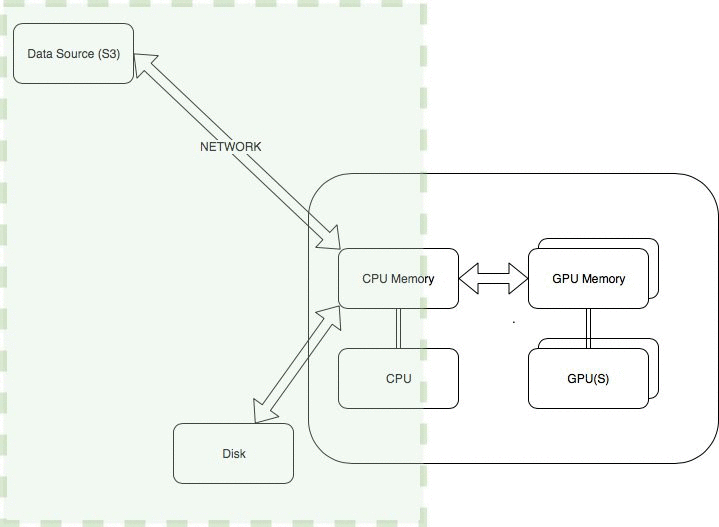
The following diagram illustrates the architecture of optimizing I/O.

The general steps usually involved in getting the data into the GPU memory are the following:
- Network operations – Download the data from Amazon Simple Storage Service (Amazon S3).
- Disk I/O – Read data from local disk into CPU memory. Local disk refers to an instance store, where storage is located on disks that are physically attached to the host computer. Amazon Elastic Block Store (Amazon EBS) volumes aren’t local resources, and involve network operations.
- Data preprocessing – The CPU generally handles any data preprocessing such as conversion or resizing. These operations might include converting images or text to tensors or resizing images.
- Data transfer into GPU memory – Copy the processed data from the CPU memory into the GPU memory.
The following sections look at optimizing these steps.
Optimizing data download over the network
In this section, we look at tips to optimize data transfer via network operations, e.g. downloading data from Amazon S3, use of file systems such as Amazon EBS & Amazon Elastic File System (Amazon EFS).
Optimizing file sizes
You can store large amounts of data in Amazon S3 at low cost. This includes data from application databases extracted through an ETL process into a JSON or CSV format or image files. One of the first steps that Amazon SageMaker does is download the files from Amazon S3, which is the default input mode called File mode.
Downloading or uploading very small files, even in parallel, is slower than larger files totaling up to the same size. For instance, if you have 2,000,000 files, where each file is 5 KB (total size = 10 GB = 2,000,000 X 5 * 1024), downloading these many tiny files can take a few hours, compared to a few minutes when downloading 2,000 files each 5 MB in size (total size = 10 GB = 2,000 X 5 * 1024 * 1024 ), even though the total download size is the same.
One of the primary reasons for this is the read/write block size. Assume that the total volume and the number of threads used for transfer is roughly the same for the large and the small files. If the transfer block size is 128 KB and the file size is 2 KB, instead of transferring 128 KB at one time, you only transfer 2 KB.
On the other hand, if the files are too large, you can’t take advantage of parallel processing to upload or download data to make it faster unless you use options such as Amazon S3 range gets to download different blocks in parallel.
Formats like MXNet RecordIO and TFRecord allow you to compress and densely pack multiple image files into a single file to avoid this trade-off. For instance, MXNet RecordIO for images recommends that images are reduced in size so you can fit at least a batch of images into CPU/GPU memory and multiple images are densely packed into a single file, so I/O operations on a tiny file don’t become a bottleneck.
As a general rule, the optimal file size ranges from 1–128 MB.
Amazon SageMaker ShardedByS3Key Amazon S3 data distribution for large datasets
During distributed training, you can also shard very large datasets across various instances. You can achieve this in an Amazon SageMaker training job by setting the parameter S3DataDistributionType to ShardedByS3Key. In this mode, if the Amazon S3 input dataset has total M objects and the training job has N instances, each instance handles M/N objects. For more information, see S3DataSource. For this use case, model training on each machine uses only the subset of training data.
Amazon SageMaker Pipe mode for large datasets
Compared to SageMaker File mode, Pipe mode allows large data to be streamed directly to your training instances from Amazon S3 instead of downloading to disk first. Pipe mode allows your code to access the data without having to wait for the entire download. Because data is never downloaded to disk and only a relatively smaller footprint is maintained in memory, data is continuously downloaded from Amazon S3 throughout each epoch. This makes it a great fit for working with very large datasets that can’t fit into the CPU memory. To take advantage of the partial raw bytes as they become available when streamed, you need your code to decode the bytes depending on the record format (such as CSV) and find the end of record to convert the partial bytes into a logical record. Amazon SageMaker TensorFlow provides built-in Pipe mode dataset readers for common formats such as text files and TFRecord. For more information, see Amazon SageMaker Adds Batch Transform Feature and Pipe Input Mode for TensorFlow Containers. If you use frameworks or libraries that don’t have built-in data readers, you could use ML-IO libraries or write your own data readers to make use of Pipe mode.
Another consequence of Pipe mode streaming is that to shuffle the data, you should use ShuffleConfig to shuffle the results of the Amazon S3 key prefix matches or lines in a manifest file and augmented manifest file. If you have one large file, you can’t rely on Amazon SageMaker to do the shuffling; you have to prefetch “N” number of batches and write your own code to shuffle depending on your ML framework.
If you can fit the entire dataset into CPU memory, File mode can be more efficient than Pipe mode. This is because if you can easily fit the entire dataset into the CPU memory, with File mode, you need to download the entire dataset into disk one time, load the entire dataset into memory one time, and repeatedly read from memory across all epochs. Reading from memory is typically much faster than network I/O, which allows you to achieve better performance.
The following section discusses how to deal with very large datasets.
Amazon FSx for Lustre or Amazon EFS for large datasets
For very large datasets, you can reduce Amazon S3 download times by using a distributed file system.
You can reduce startup times using Amazon FSx for Lustre on Amazon SageMaker while maintaining the data in Amazon S3. For more information, see Speed up training on Amazon SageMaker using Amazon FSx for Lustre and Amazon EFS file systems.
The first time you run a training job, FSx for Lustre automatically copies data from Amazon S3 and makes it available to Amazon SageMaker. Additionally, you can use the same FSx for Lustre file system for subsequent iterations of training jobs on Amazon SageMaker, which prevents repeated downloads of common Amazon S3 objects. Because of this, FSx for Lustre has the most benefit for training jobs that have training sets in Amazon S3 and in workflows where training jobs must be run several times using different training algorithms or parameters to see which gives the best result.
If you already have your training data on Amazon Elastic File System (Amazon EFS), you can also use Amazon EFS with Amazon SageMaker. For more information, see Speed up training on Amazon SageMaker using Amazon FSx for Lustre and Amazon EFS file systems.
One thing to consider while using this option is file size. If the file sizes are too small, the I/O performance is likely to be slower due to factors such as transfer block size.
Amazon SageMaker instances with local NVMe-based SSD storage
Some of the Amazon SageMaker GPU instances, such as the ml.p3dn.24xlarge and ml.g4dn, provide local NVMe-based SSD storage instead of EBS volumes. For instance, the ml.p3dn.24xlarge instances have 1.8 TB of local NVMe-based SSD storage. The use of local NVMe-based SSD storage means that after training data is downloaded from Amazon S3 to a local disk storage, the disk I/0 is much faster than reading from network resources such as EBS volumes or Amazon S3. This allows you to achieve faster training times when the training data size can fit into the local NVMe-based storage.
Optimizing data loading and preprocessing
In the preceding section, we described how to download data from sources like Amazon S3 efficiently. In this section, we discuss how to increase parallelism and make commonly used functions as lean as possible to make data loading more efficient.
Multiple workers for loading and processing data
TensorFlow, MXNet Gluon, and PyTorch provide data loader libraries for loading data in parallel. In the following PyTorch example, increasing the number of workers allows more workers to process items in parallel. As a general rule, you may scale up from a single worker to approximately one less than the number of CPUs. Generally, each worker represents one process and uses Python multiprocessing, although the implementation details can vary from framework to framework. The use of multiprocessing sidesteps the Python Global Interpreter Lock (GIL) to fully use all the CPUs in parallel, but it also means that memory utilization increases proportionally to the number of workers because each process has its own copy of the objects in memory. You might see out of memory exceptions as you start to increase the number of workers, in which case you should use an instance that has more CPU memory where applicable.
To understand the effect of using the workers, we present the following example dataset. In this dataset, the __get_item__ operation sleeps for 1 second, to emulate some latency in reading the next record:
class MockDatasetSleep(Dataset):
    """
    Simple mock dataset to understand the use of workers
    """

    def __init__(self, num_cols, max_records=32):
        super(MockDatasetSleep).__init__()
        self.max_records = max_records
        self.num_cols = num_cols

        # Initialising mock x and y
        self.x = np.random.uniform(size=self.num_cols)
        self.y = np.random.normal()

        print("Initialised")


    def __len__(self):
        return self.max_records

    def __getitem__(self, idx):
        curtime = datetime.datetime.now()

        # Emulate a slow operation
        sleep_seconds = 1

        time.sleep(sleep_seconds)
        print("{}: retrieving item {}".format(curtime, idx))

        return self.x, self.y
As an example, create a data loader instance with only a single worker:
# One worker
num_workers = 1
torch.utils.data.DataLoader(MockDatasetSleep(), batch_size=batch_size, shuffle=True, num_workers=num_workers)
When you use a single worker, you see items retrieved one by one, with a 1-second delay to retrieve each item:
15:39:58.833644: retrieving item 0
15:39:59.834420: retrieving item 6
15:40:00.834861: retrieving item 8
15:40:01.835350: retrieving item 5
If you increase the number of workers to 3 workers on an instance, that has at least 4 CPUs to ensure maximum parallel processing. See the following code:
# You may need to lower the number of workers if you encounter out of memory exceptions or move to a instance with more memory
num_workers = os.cpu_count() - 1
torch.utils.data.DataLoader(train_dataset, batch_size=batch_size, shuffle=True, num_workers=num_workers)
In this example dataset, you can see that the three workers are attempting to retrieve three items in parallel, and it takes approximately 1 second for the operation to complete and the next three items are retrieved:
16:03:21.980084: retrieving item 8
16:03:21.981769: retrieving item 10
16:03:21.981690: retrieving item 25

16:03:22.980437: retrieving item 0
16:03:22.982118: retrieving item 7
16:03:22.982339: retrieving item 21
In this demo notebook example, we use the Caltech-256 dataset, which has approximately 30,600 images, using ResNet 50. In the Amazon SageMaker training job, we use a single ml.p3.2xlarge instance, which comes with 1 GPU and 8 vCPUs. With just one worker, it took 260 seconds per epoch processing approximately 100 images per second in a single GPU. With seven workers, it took 96 seconds per epoch processing approximately 300 images per second, a performance improvement that is three times faster.
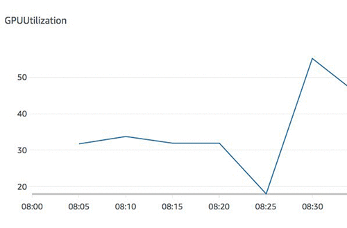
The following graph shows the metric GPUUtilization for a single worker with peak utilization 50%.

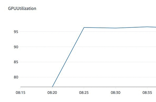
The following graph shows the metric GPUUtilization for multiple workers, which has an average utilization of 95%.

Minor changes to num_workers can speed up data loading and therefore allow the GPUs to train faster because they spend less time waiting for data. This shows how optimizing the I/O performance in data loaders can improve GPU utilization.
You should only train on multi-GPU or multi-host distributed GPU training after you optimize usage on a single GPU. Therefore, it’s absolutely critical to measure and maximize utilization on a single GPU before moving on to distributed training.
Optimizing frequently used functions
Minimizing expensive operations while retrieving each record item where possible can improve training performance regardless of the GPU or CPU. You can optimize frequently used functions in many ways, such as using the right data structures.
In the demo notebook example, the naive implementation loads the image file and resizes during each item, as shown in the following code. We optimize this function by preprocessing the Caltech 256 dataset to resize the images ahead of time and save a pickled version of image files. The __getitem__ function only attempts to randomly crop the image, which makes the __getitem__ function quite lean. The GPU spends less time waiting for the CPU to preprocess the data, which makes the data available to the GPU faster. See the following code:
# Naive implementation
def __getitem__(self, idx):
        curtime = datetime.datetime.now()

        self.logger.debug("{}: retrieving item {}".format(curtime, idx))

        image, label = self.images[idx], self.labels[idx]

        # Convert to PIL image to apply transformations
        # This could be faster if handled in a preprocessing step
        image = Image.open(image)
        if image.getbands()[0] == 'L':
            image = image.convert('RGB')

        # Apply transformation at each get item including resize, random crop
        image = self.transformer(image)
        self.logger.debug("{}: completed item {}".format(datetime.datetime.now(), idx))

        return image, label

# Optimised implementation
def __getitem__(self, idx):
        curtime = datetime.datetime.now()

        self.logger.debug("{}: retrieving item {}".format(curtime, idx))

        image, label = self.images[idx], self.labels[idx]

        # Apply transformation at each get item - random crop
        image = self.transformer(image)

        self.logger.debug("{}: completed item {}".format(datetime.datetime.now(), idx))

        return image, label
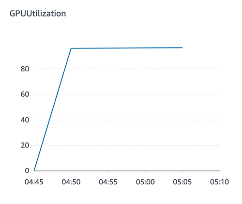
Even with this simple change, we could complete an epoch in 96 seconds, with approximately 300 images per second, which is three times faster than the unoptimized dataset with a single worker. If we increase the number of workers, it makes very little difference to the GPU utilization because the data loading process is no longer the bottleneck.
In some use cases, you may have to increase the number of workers and optimize the code to maximize the GPU utilization.
The following graph shows GPU utilization with a single worker using the optimized dataset.

The following graph shows GPU utilization with the unoptimized dataset.

Know your ML framework
The data loading libraries for the respective deep learning framework can provide additional options to optimize data loading, including Tensorflow data loader, MXNet, and PyTorch data loader. You should understand the parameters for data loaders and libraries that best work for your use case and the trade-offs involved. Some of these options include:
- CPU pinned memory – Allows you to accelerate data transfer from the CPU (host) memory to the GPU (device) memory. This performance gain is obtained by directly allocating page-locked (or pinned) memory instead of allocating a paged memory first and copying data from CPU paged to CPU pinned memory to transfer data to the GPU. Enabling CPU pinned memory in the data loader is available in PyTorch and MXNet. The trade-off to consider is out of memory exceptions are more likely to occur when requesting pinned CPU memory instead of paged memory.
- Modin – This lightweight parallel processing data frame allows you to perform Pandas dataframe-like operations in parallel so you can fully utilize all the CPUs on your machine. Modin can use different types of parallel processing frameworks such as Dask and Ray.
- CuPy – This open-source matrix library, similar to NumPy, provides GPU accelerated computing with Python.
Heuristics to identify I/O bottlenecks
Amazon SageMaker provides Amazon CloudWatch metrics such as GPU, CPU, and disk utilization during training. For more information, see Monitor Amazon SageMaker with Amazon CloudWatch.
The following heuristics identify I/O-related performance issues using the out-of-the-box metrics:
- If your training job takes a very long time to start, most of the time is spent downloading the data. You should look at ways to optimize downloading from Amazon S3, as detailed earlier.
- If the GPU utilization is low but the disk or the CPU utilization is high, data loading or preprocessing could be potential bottlenecks. You might want to preprocess the data well ahead of training, if possible. You could also optimize the most frequently used functions, as demonstrated earlier.
- If the GPU utilization is low and the CPU and disk utilization is continuously low but not zero, despite having a large enough dataset, it could mean that your code isn’t utilizing the underlying resources effectively. If you notice that the CPU memory utilization is also low, a quick way to potentially boost performance is to increase the number of workers in the data loader API of your deep learning framework.
Conclusion
In summary, you can see how the foundations of data loading and processing affect GPU utilization, and how you can improve GPU performance by resolving I/O- or network-related bottlenecks. It’s important to address these bottlenecks before moving to advance topics such as multi-GPU or distributed training.
For more information to help you get started with Amazon SageMaker, see the following:
- Amazon SageMaker examples – GitHub repo
- TensorFlow – Better performance with the tf.data API
- MXNet – Designing Efficient Data Loaders for Deep Learning
- PyTorch data loader – TORCH.UTILS.DATA
About the Author
 Aparna Elangovan is a Artificial Intelligence & Machine Learning Prototyping Engineer at AWS, where she helps customers develop deep learning applications.
