Data quality is an important topic for virtually all teams and systems deriving insights from data, especially teams and systems using machine learning (ML) models. Supervised ML is the task of learning a function that maps an input to an output based on examples of input-output pairs. For a supervised ML algorithm to effectively learn this mapping, the input-output pairs must be accurately labeled, which makes data labeling a crucial step in any supervised ML task.
Supervised ML is commonly used in the computer vision space. You can train an algorithm to perform a variety of tasks, including image classification, bounding box detection, and semantic segmentation, among many others. Computer vision annotation tools, like those available in Amazon SageMaker Ground Truth (Ground Truth), simplify the process of creating labels for computer vision algorithms and encourage best practices, resulting in high-quality labels.
To ensure quality, humans must be involved at some stage to either annotate or verify the assets. However, human labelers are often expensive, so it’s important to use them cost-effectively. There is no industry-wide standard for automatically monitoring the quality of annotations during the labeling process of images (or videos or point clouds), so human verification is the most common solution.
The process for human verification of labels involves expert annotators (verifiers) verifying a sample of the data labeled by a primary annotator where the experts correct (overturn) any errors in the labels. You can often find candidate samples that require label verification by using ML methods. In some scenarios, you need the same images, videos, or point clouds to be labeled and processed by multiple labelers to determine ground truth when there is ambiguity. Ground Truth accomplishes this through annotation consolidation to get agreement on what the ground truth is based on multiple responses.
In computer vision, we often deal with tasks that contain a temporal dimension, such as video and LiDAR sensors capturing sequential frames. Labeling this kind of sequential data is complex and time consuming. The goal of this blog post is to reduce the total number of frames that need human review by performing automated quality checks in multi-object tracking (MOT) time series data like video object tracking annotations while maintaining data quality at scale. The quality initiative in this blog post proposes science-driven methods that take advantage of the sequential nature of these inputs to automatically identify potential outlier labels. These methods enable you to a) objectively track data labeling quality for Ground Truth video, b) use control mechanisms to achieve and maintain quality targets, and c) optimize costs to obtain high-quality data.
We will walk through an example situation in which a large video dataset has been labeled by primary human annotators for a ML system and demonstrate how to perform automatic quality assurance (QA) to identify samples that may not be labeled properly. How can this be done without overwhelming a team’s limited resources? We’ll show you how using Ground Truth and Amazon SageMaker.
Background
Data annotation is, typically, a manual process in which the annotator follows a set of guidelines and operates in a “best-guess” manner. Discrepancies in labeling criteria between annotators can have an effect on label quality, which may impact algorithm inference performance downstream.
For sequential inputs like video at a high frame rate, it can be assumed that a frame at time t will be very similar to a frame at time t+1. This extends to the labeled objects in the frames and allows large deviations between labels across labels to be considered outliers, which can be identified with statistical metrics. Auditors can be directed to pay special attention to these outlier frames in the verification process.
A common theme in feedback from customers is the desire to create a standard methodology and framework to monitor annotations from Ground Truth and identify frames with low-quality annotations for auditing purposes. We propose this framework to allow you to measure the quality on a certain set of metrics and take action — for example, by sending those specific frames for relabeling using Ground Truth or Amazon Augmented AI (Amazon A2I).
The following table provides a glossary of terms frequently used in this post.
| Term | Meaning |
| Annotation | The process whereby a human manually captures metadata related to a task. An example would be drawing the outline of the products in a still image. |
| SageMaker Ground Truth | Ground Truth handles the scheduling of various annotation tasks and collecting the results. It also supports defining labor pools and labor requirements for performing the annotation tasks. |
| IoU | The intersection over union (IoU) ratio measures overlap between two regions of interest in an image. This measures how good our object detector prediction is with the ground truth (the real object boundary). |
| Detection rate | The number of detected boxes/number of ground truth boxes. |
| Annotation pipeline | The complete end-to-end process of capturing a dataset for annotation, submitting the dataset for annotation, performing the annotation, performing quality checks and adjusting incorrect annotations. |
| Source data | The MOT17 dataset. |
| Target data | The unified ground truth dataset. |
Evaluation metrics
This is an exciting open area of research for quality validation of annotations using statistical approaches, and the following quality metrics are often used to perform statistical validation.
Intersection over union (IoU)
IoU is the overlap between the ground truth and the prediction for each frame and the percentage of overlap between two bounding boxes. A high IoU combined with a low Hausdorff Distance indicates that a source bounding box corresponds well with a target bounding box in geometric space. These parameters may also indicate a skew in imagery. A low IoU may indicate quality conflicts between bounding boxes.

In the preceding equation bp is predicted bounding box and bgt is the ground truth bounding box.
Center Loss
Center loss is the distance between bounding box centers:

In the preceding equation (xp>,yp) is the center of predicted bounding box and (xgt,ygt) is the center of the ground truth bounding box.
IoU distribution
If the mean, median, and mode of an object’s IoU is drastically different than other objects, we may want to flag the object in question for manual auditing. We can use visualizations like heat maps for a quick understanding of object-level IoU variance.
MOT17 Dataset
The Multi Object Tracking Benchmark is a commonly used benchmark for multiple target tracking evaluation. They have a variety of datasets for training and evaluating multi-object tracking models available. For this post, we use the MOT17 dataset for our source data, which is based around detecting and tracking a large number of vehicles.
Solution
To run and customize the code used in this blog post, use the notebook Ground_Truth_Video_Quality_Metrics.ipynb in the Amazon SageMaker Examples tab of a notebook instance, under Ground Truth Labeling Jobs. You can also find the notebook on GitHub.
Download MOT17 dataset
Our first step is to download the data, which takes a few minutes, unzip it, and send it to Amazon Simple Storage Service (Amazon S3) so we can launch audit jobs. See the following code:
# Grab our data this will take ~5 minutes
!wget https://motchallenge.net/data/MOT17.zip -O /tmp/MOT17.zip

# unzip our data
!unzip -q /tmp/MOT17.zip -d MOT17
!rm /tmp/MOT17.zip
View MOT17 annotations
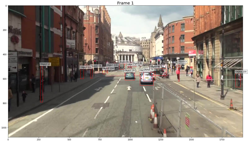
Now let’s look at what the existing MOT17 annotations look like.
In the following image, we have a scene with a large number of cars and pedestrians on a street. The labels include both bounding box coordinates as well as unique IDs for each object, or in this case cars, being tracked.
Evaluate our labels
For demonstration purposes, we’ve labeled three vehicles in one of the videos and inserted a few labeling anomalies into the annotations. Although human labelers tend to be accurate, they’re subject to conditions like distraction and fatigue, which can affect label quality. If we use automated methods to identify annotator mistakes and send directed recommendations for frames and objects to fix, we can make the label auditing process more accurate and efficient. If a labeler only has to focus on a few frames instead of a deep review of the entire scene, they can drastically improve speed and reduce cost.
Analyze our tracking data
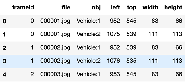
Let’s put our tracking data into a form that’s easier to analyze.
We use a function to take the output JSON from Ground Truth and turn our tracking output into a dataframe. We can use this to plot values and metrics that will help us understand how the object labels move through our frames. See the following code:
# generate dataframes
lab_frame_real = create_annot_frame(tlabels['tracking-annotations'])
lab_frame_real.head()
Plot progression
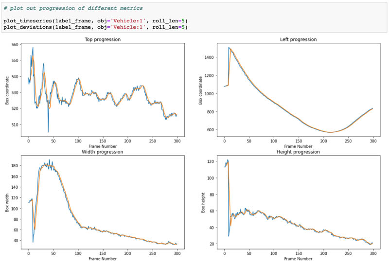
Let’s start with some simple plots. The following plots illustrate how the coordinates of a given object progress through the frames of your video. Each bounding box has a left and top coordinate, representing the top-left point of the bounding box. We also have height and width values that let us determine the other three points of the box.
In the following plots, the blue lines represent the progression of our four values (top coordinate, left coordinate, width, and height) through the video frames and the orange lines represent a rolling average of the values from the previous five frames. Because a video is a sequence of frames, if we have a video that has five frames per second or more, the objects within the video (and the bounding boxes drawn around them) should have some amount of overlap between frames. In our video, we have vehicles driving at a normal pace so our plots should show a relatively smooth progression.
We can also plot the deviation between the rolling average and the actual values of bounding box coordinates. We’ll likely want to look at frames where the actual value deviates substantially from the rolling average.
Plot box sizes
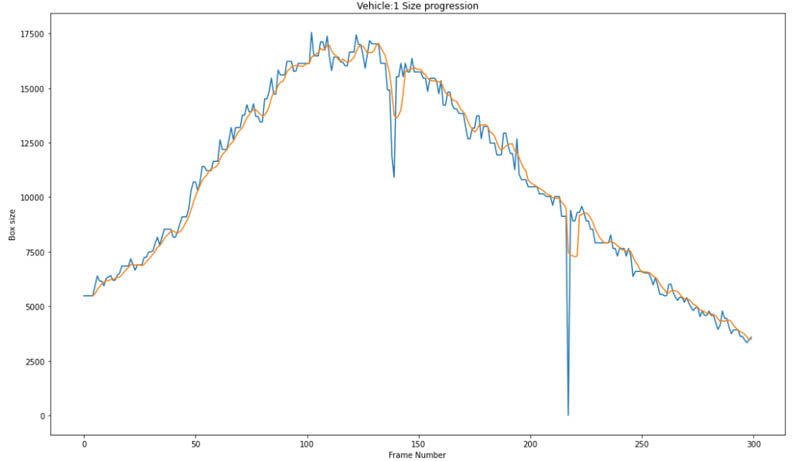
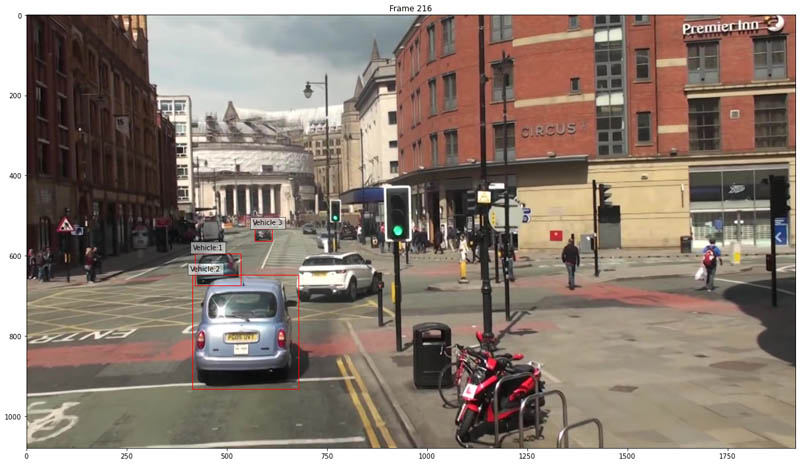
Let’s combine the width and height values to look at how the size of the bounding box for a given object progresses through the scene. For Vehicle 1, we intentionally reduced the size of the bounding box on frame 139 and restored it on frame 141. We also removed a bounding box on frame 217. We can see both of these flaws reflected in our size progression plots.
Box size differential
Let’s now look at how the size of the box changes from frame to frame by plotting the actual size differential. This allows us to get a better idea of the magnitude of these changes. We can also normalize the magnitude of the size changes by dividing the size differentials by the sizes of the boxes. This lets us express the differential as a percentage change from the original size of the box. This makes it easier to set thresholds beyond which we can classify this frame as potentially problematic for this object bounding box. The following plots visualize both the absolute size differential and the size differential as a percentage. We can also add lines representing where the bounding box changed by more than 20% in size from one frame to the next.

View the frames with the largest size differential
Now that we have the indexes for the frames with the largest size differential, we can view them in sequence. If we look at the following frames, we can see for Vehicle 1 we were able to identify frames where our labeler made a mistake. Frame 217 was flagged because there was a large difference between frame 216 and the subsequent frame, frame 217.
Rolling IoU
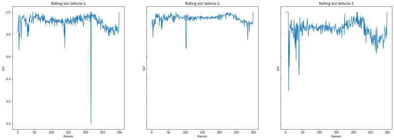
IoU is a commonly used evaluation metric for object detection. We calculate it by dividing the area of overlap between two bounding boxes by the area of union for two bounding boxes. Although it’s typically used to evaluate the accuracy of a predicted box against a ground truth box, we can use it to evaluate how much overlap a given bounding box has from one frame of a video to the next.
Because our frames differ, we don’t expect a given bounding box for a single object to have 100% overlap with the corresponding bounding box from the next frame. However, depending on the frames per second for the video, there often is only a small amount of change in one from to the next because the time elapsed between frames is only a fraction of a second. For higher FPS video, we can expect a substantial amount of overlap between frames. The MOT17 videos are all shot at 25 FPS, so these videos qualify. Operating with this assumption, we can use IoU to identify outlier frames where we see substantial differences between a bounding box in one frame to the next. See the following code:
# calculate rolling intersection over union
def calc_frame_int_over_union(annot_frame, obj, i):
    lframe_len = max(annot_frame['frameid'])
    annot_frame = annot_frame[annot_frame.obj==obj]
    annot_frame.index = list(np.arange(len(annot_frame)))
    coord_vec = np.zeros((lframe_len+1,4))
    coord_vec[annot_frame['frameid'].values, 0] = annot_frame['left']
    coord_vec[annot_frame['frameid'].values, 1] = annot_frame['top']
    coord_vec[annot_frame['frameid'].values, 2] = annot_frame['width']
    coord_vec[annot_frame['frameid'].values, 3] = annot_frame['height']
    boxA = [coord_vec[i,0], coord_vec[i,1], coord_vec[i,0] + coord_vec[i,2], coord_vec[i,1] + coord_vec[i,3]]
    boxB = [coord_vec[i+1,0], coord_vec[i+1,1], coord_vec[i+1,0] + coord_vec[i+1,2], coord_vec[i+1,1] + coord_vec[i+1,3]]
    return bb_int_over_union(boxA, boxB)
# create list of objects
objs = list(np.unique(label_frame.obj))
# iterate through our objects to get rolling IoU values for each
iou_dict = {}
for obj in objs:
    iou_vec = np.ones(len(np.unique(label_frame.frameid)))
    ious = []
    for i in label_frame[label_frame.obj==obj].frameid[:-1]:
        iou = calc_frame_int_over_union(label_frame, obj, i)
        ious.append(iou)
        iou_vec[i] = iou
    iou_dict[obj] = iou_vec

fig, ax = plt.subplots(nrows=1,ncols=3, figsize=(24,8), sharey=True)
ax[0].set_title(f'Rolling IoU {objs[0]}')
ax[0].set_xlabel('frames')
ax[0].set_ylabel('IoU')
ax[0].plot(iou_dict[objs[0]])
ax[1].set_title(f'Rolling IoU {objs[1]}')
ax[1].set_xlabel('frames')
ax[1].set_ylabel('IoU')
ax[1].plot(iou_dict[objs[1]])
ax[2].set_title(f'Rolling IoU {objs[2]}')
ax[2].set_xlabel('frames')
ax[2].set_ylabel('IoU')
ax[2].plot(iou_dict[objs[2]])
The following plots show our results:
Identify and visualize low overlap frames
Now that we have calculated our intersection over union for our objects, we can identify objects below an IoU threshold we set. Let’s say we want to identify frames where the bounding box for a given object has less than 50% overlap. We can use the following code:
## ID problem indices
iou_thresh = 0.5
vehicle = 1 # because index starts at 0, 0 -> vehicle:1, 1 -> vehicle:2, etc.
# use np.where to identify frames below our threshold.
inds = np.where(np.array(iou_dict[objs[vehicle]]) < iou_thresh)[0]
worst_ind = np.argmin(np.array(iou_dict[objs[vehicle]]))
print(objs[vehicle],'worst frame:', worst_ind)
Visualize low overlap frames
Now that we have identified our low overlap frames, let’s view them. We can see for Vehicle:2, there is an issue on frame 102, compared to frame 101.
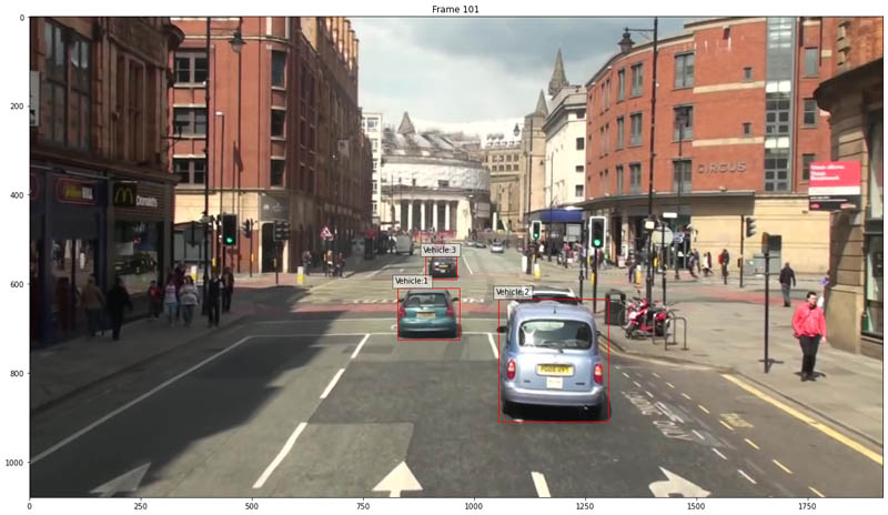
The annotator made a mistake and the bounding box for Vehicle:2 does not go low enough and clearly needs to be extended.
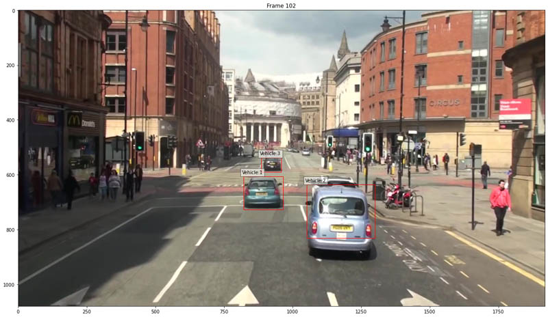
Thankfully our IoU metric was able to identify this!
Embedding comparison
The two preceding methods work because they’re simple and are based on the reasonable assumption that objects in high FPS video don’t move too much from frame to frame. They can be considered more classical methods of comparison. Can we improve upon them? Let’s try something more experimental.
We can use a deep learning method to identify outliers is to generate embeddings for our bounding box crops with an image classification model like ResNet and compare these across frames. Convolutional neural network image classification models have a final fully connected layer using a softmax or scaling activation function that outputs probabilities. If we remove the final layer of our network, our predictions will instead be the image embedding that is essentially the neural network’s representation of the image. If we isolate our objects by cropping our images, we can compare the representations of these objects across frames to see if we can identify any outliers.
We can use a ResNet18 model from Torchhub that was trained on ImageNet. Because ImageNet is a very large and generic dataset, the network over time was able to learn information regarding images that allow it to classify them into different categories. While a neural network more finely tuned on vehicles would likely perform better, a network trained on a large dataset like ImageNet should have learned enough information to give us some indication if images are similar.
The following code shows our crops:
def plot_crops(obj = 'Vehicle:1', start=0):
    fig, ax = plt.subplots(nrows=1, ncols=5, figsize=(20,12))
    for i,a in enumerate(ax):
        a.imshow(img_crops[i+start][obj])
        a.set_title(f'Frame {i+start}')
plot_crops(start=1)
The following image compares the crops in each frame:

Let’s compute the distance between our sequential embeddings for a given object:
def compute_dist(img_embeds, dist_func=distance.euclidean, obj='Vehicle:1'):
    dists = []
    inds = []
    for i in img_embeds:
        if (i>0)&(obj in list(img_embeds[i].keys())):
            if (obj in list(img_embeds[i-1].keys())):
                dist = dist_func(img_embeds[i-1][obj],img_embeds[i][obj]) # distance  between frame at t0 and t1
                dists.append(dist)
                inds.append(i)
    return dists, inds
obj = 'Vehicle:2'
dists, inds = compute_dist(img_embeds, obj=obj)

# look for distances that are 2 standard deviation greater than the mean distance
prob_frames = np.where(dists>(np.mean(dists)+np.std(dists)*2))[0]
prob_inds = np.array(inds)[prob_frames]
print(prob_inds)
print('The frame with the greatest distance is frame:', inds[np.argmax(dists)])
Let’s look at the crops for our problematic frames. We can see we were able to catch the issue on frame 102 where the bounding box was off-center.

Combine the metrics
Now that we have explored several methods for identifying anomalous and potentially problematic frames, let’s combine them and identify all of those outlier frames (see the following code). Although we might have a few false positives, these tend to be areas with a lot of action that we might want our annotators to review regardless.
def get_problem_frames(lab_frame, flawed_labels, size_thresh=.25, iou_thresh=.4, embed=False, imgs=None, verbose=False, embed_std=2):
    """
    Function for identifying potentially problematic frames using bounding box size, rolling IoU, and optionally embedding comparison.
    """
    if embed:
        model = torch.hub.load('pytorch/vision:v0.6.0', 'resnet18', pretrained=True)
        model.eval()
        modules=list(model.children())[:-1]
        model=nn.Sequential(*modules)

    frame_res = {}
    for obj in list(np.unique(lab_frame.obj)):
        frame_res[obj] = {}
        lframe_len = max(lab_frame['frameid'])
        ann_subframe = lab_frame[lab_frame.obj==obj]
        size_vec = np.zeros(lframe_len+1)
        size_vec[ann_subframe['frameid'].values] = ann_subframe['height']*ann_subframe['width']
        size_diff = np.array(size_vec[:-1])- np.array(size_vec[1:])
        norm_size_diff = size_diff/np.array(size_vec[:-1])
        norm_size_diff[np.where(np.isnan(norm_size_diff))[0]] = 0
        norm_size_diff[np.where(np.isinf(norm_size_diff))[0]] = 0
        frame_res[obj]['size_diff'] = [int(x) for x in size_diff]
        frame_res[obj]['norm_size_diff'] = [int(x) for x in norm_size_diff]
        try:
            problem_frames = [int(x) for x in np.where(np.abs(norm_size_diff)>size_thresh)[0]]
            if verbose:
                worst_frame = np.argmax(np.abs(norm_size_diff))
                print('Worst frame for',obj,'in',frame, 'is: ',worst_frame)
        except:
            problem_frames = []
        frame_res[obj]['size_problem_frames'] = problem_frames
        iou_vec = np.ones(len(np.unique(lab_frame.frameid)))
        for i in lab_frame[lab_frame.obj==obj].frameid[:-1]:
            iou = calc_frame_int_over_union(lab_frame, obj, i)
            iou_vec[i] = iou

        frame_res[obj]['iou'] = iou_vec.tolist()
        inds = [int(x) for x in np.where(iou_vec<iou_thresh)[0]]
        frame_res[obj]['iou_problem_frames'] = inds

        if embed:
            img_crops = {}
            img_embeds = {}
            for j,img in tqdm(enumerate(imgs)):
                img_arr = np.array(img)
                img_embeds[j] = {}
                img_crops[j] = {}
                for i,annot in enumerate(flawed_labels['tracking-annotations'][j]['annotations']):
                    try:
                        crop = img_arr[annot['top']:(annot['top']+annot['height']),annot['left']:(annot['left']+annot['width']),:]
                        new_crop = np.array(Image.fromarray(crop).resize((224,224)))
                        img_crops[j][annot['object-name']] = new_crop
                        new_crop = np.reshape(new_crop, (1,224,224,3))
                        new_crop = np.reshape(new_crop, (1,3,224,224))
                        torch_arr = torch.tensor(new_crop, dtype=torch.float)
                        with torch.no_grad():
                            emb = model(torch_arr)
                        img_embeds[j][annot['object-name']] = emb.squeeze()
                    except:
                        pass

            dists = compute_dist(img_embeds, obj=obj)
            # look for distances that are 2+ standard deviations greater than the mean distance
            prob_frames = np.where(dists>(np.mean(dists)+np.std(dists)*embed_std))[0]
            frame_res[obj]['embed_prob_frames'] = prob_frames.tolist()

    return frame_res

# if you want to add in embedding comparison, set embed=True
num_images_to_validate = 300
embed = False
frame_res = get_problem_frames(label_frame, flawed_labels, size_thresh=.25, iou_thresh=.5, embed=embed, imgs=imgs[:num_images_to_validate])

prob_frame_dict = {}
all_prob_frames = []
for obj in frame_res:
    prob_frames = list(frame_res[obj]['size_problem_frames'])
    prob_frames.extend(list(frame_res[obj]['iou_problem_frames']))
    if embed:
        prob_frames.extend(list(frame_res[obj]['embed_prob_frames']))
    all_prob_frames.extend(prob_frames)

prob_frame_dict = [int(x) for x in np.unique(all_prob_frames)]
prob_frame_dict
Launch a directed audit job
Now that we’ve identified our problematic annotations, we can launch a new audit labeling job to review identified outlier frames. We can do this via the SageMaker console, but when we want to launch jobs in a more automated fashion, using the boto3 API is very helpful.
Generate manifests
SageMaker Ground Truth operates using manifests. When using a modality like image classification, a single image corresponds to a single entry in a manifest and a given manifest will contains paths for all of the images to be labeled in a single manifest. For videos, because we have multiple frames per video and we can have multiple videos in a single manifest, this is organized instead by using a JSON sequence file for each video that contains all the paths for our frames. This allows a single manifest to contain multiple videos for a single job. For example, the following code:
# create manifest
man_dict = {}
for vid in all_vids:
    source_ref = f"s3://{bucket}/tracking_manifests/{vid.split('/')[-1]}_seq.json"
    annot_labels = f"s3://{bucket}/tracking_manifests/SeqLabel.json"
    manifest = {
        "source-ref": source_ref,
        'Person':annot_labels,
        "Person-metadata":{"class-map": {"1": "Pedestrian"},
                         "human-annotated": "yes",
                         "creation-date": "2020-05-25T12:53:54+0000",
                         "type": "groundtruth/video-object-tracking"}
    }
    man_dict[vid] = manifest

# save videos as individual jobs
for vid in all_vids:
    with open(f"tracking_manifests/{vid.split('/')[-1]}.manifest", 'w') as f:
        json.dump(man_dict[vid],f)

# put multiple videos in a single manifest, with each job as a line
# with open(f"/home/ec2-user/SageMaker/tracking_manifests/MOT17.manifest", 'w') as f:
#     for vid in all_vids:
#         f.write(json.dumps(man_dict[vid]))
#         f.write('n')

print('Example manifest: ', manifest)
The following is our manifest file:
Example manifest: {'source-ref': 's3://smgt-qa-metrics-input-322552456788-us-west-2/tracking_manifests/MOT17-13-SDP_seq.json', 'Person': 's3://smgt-qa-metrics-input-322552456788-us-west-2/tracking_manifests/SeqLabel.json', 'Person-metadata': {'class-map': {'1': 'Vehicle'}, 'human-annotated': 'yes', 'creation-date': '2020-05-25T12:53:54+0000', 'type': 'groundtruth/video-object-tracking'}}Launch jobs
We can use this template for launching labeling jobs (see the following code). For the purposes of this post, we already have labeled data, so this isn’t necessary, but if you want to label the data yourself, you can do so using a private workteam.
# generate jobs
job_names = []
outputs = []
# for vid in all_vids:
LABELING_JOB_NAME = f"mot17-tracking-adjust-{int(time.time()} "
task = 'AdjustmentVideoObjectTracking'
job_names.append(LABELING_JOB_NAME)
INPUT_MANIFEST_S3_URI = f's3://{bucket}/tracking_manifests/MOT20-01.manifest'
createLabelingJob_request = {
  "LabelingJobName": LABELING_JOB_NAME,
  "HumanTaskConfig": {
    "AnnotationConsolidationConfig": {
      "AnnotationConsolidationLambdaArn": f"arn:aws:lambda:us-east-1:432418664414:function:ACS-{task}"
    }, # changed us-west-2 to us-east-1
    "MaxConcurrentTaskCount": 200,
    "NumberOfHumanWorkersPerDataObject": 1,
    "PreHumanTaskLambdaArn": f"arn:aws:lambda:us-east-1:432418664414:function:PRE-{task}",
    "TaskAvailabilityLifetimeInSeconds": 864000,
    "TaskDescription": f"Please draw boxes around vehicles, with a specific focus on the following frames {prob_frame_dict}",
    "TaskKeywords": [
      "Image Classification",
      "Labeling"
    ],
    "TaskTimeLimitInSeconds": 7200,
    "TaskTitle": LABELING_JOB_NAME,
    "UiConfig": {
      "HumanTaskUiArn": f'arn:aws:sagemaker:us-east-1:394669845002:human-task-ui/VideoObjectTracking'
    },
    "WorkteamArn": WORKTEAM_ARN
  },
  "InputConfig": {
    "DataAttributes": {
      "ContentClassifiers": [
        "FreeOfPersonallyIdentifiableInformation",
        "FreeOfAdultContent"
      ]
    },
    "DataSource": {
      "S3DataSource": {
        "ManifestS3Uri": INPUT_MANIFEST_S3_URI
      }
    }
  },
  "LabelAttributeName": "Person-ref",
  "LabelCategoryConfigS3Uri": LABEL_CATEGORIES_S3_URI,
  "OutputConfig": {
    "S3OutputPath": f"s3://{bucket}/gt_job_results"
  },
  "RoleArn": role,
  "StoppingConditions": {
    "MaxPercentageOfInputDatasetLabeled": 100
  }
}
print(createLabelingJob_request)
out = sagemaker_cl.create_labeling_job(**createLabelingJob_request)
outputs.append(out)
print(out)
Conclusion
In this post, we introduced how to measure the quality of sequential annotations, namely video multi-frame object tracking annotations, using statistical analysis and various quality metrics (IoU, rolling IoU and embedding comparisons). In addition, we walked through how to flag frames that aren’t labeled properly using these quality metrics and send those frames for verification or audit jobs using SageMaker Ground Truth to generate a new version of the dataset with more accurate annotations. We can perform quality checks on the annotations for video data using this approach or similar approaches such as 3D IoU for 3D point cloud data in automated manner at scale with reduction in the number of frames for human audit.
Try out the notebook and add your own quality metrics for different task types supported by SageMaker Ground Truth. With this process in place, you can generate high-quality datasets for a wide range of business use cases in a cost-effective manner without compromising the quality of annotations.
For more information about labeling with Ground Truth, see Easily perform bulk label quality assurance using Amazon SageMaker Ground Truth.
References
- https://en.wikipedia.org/wiki/Hausdorff_distance
- https://aws.amazon.com/blogs/machine-learning/easily-perform-bulk-label-quality-assurance-using-amazon-sagemaker-ground-truth/
About the Authors
 Vidya Sagar Ravipati is a Deep Learning Architect at the Amazon ML Solutions Lab, where he leverages his vast experience in large-scale distributed systems and his passion for machine learning to help AWS customers across different industry verticals accelerate their AI and cloud adoption. Previously, he was a Machine Learning Engineer in Connectivity Services at Amazon who helped to build personalization and predictive maintenance platforms.
 Isaac Privitera is a Machine Learning Specialist Solutions Architect and helps customers design and build enterprise-grade computer vision solutions on AWS. Isaac has a background in using machine learning and accelerated computing for computer vision and signals analysis. Isaac also enjoys cooking, hiking, and keeping up with the latest advancements in machine learning in his spare time.
