TL;DR: We demonstrate the use of PyTorch with FairScale’s FullyShardedDataParallel (FSDP) API in writing large vision transformer models. We discuss our techniques for scaling and optimizing these models on a GPU cluster. The goal of this platform scaling effort is to enable research at scale. This blog does not discuss model accuracy, new model architectures, or new training recipes.
1. Introduction
Latest vision research [1, 2] demonstrates model scaling as a promising research direction. In this project, we aim to enable our platforms to train massive vision transformer (ViT) [3] models. We present our work on scaling the largest trainable ViT from 1B to 120B parameters in FAIR vision platforms. We wrote ViT in PyTorch and leveraged its support for large-scale, distributed training on a GPU cluster.
In the rest of this blog, we will first discuss the main challenges, namely scalability, optimization, and numerical stability. Then we will discuss how we tackle them with techniques including data and model parallelism, automatic mixed precision, kernel fusion, and bfloat16. Finally, we present our results and conclude.
2. Main Challenges
2.1 Scalability
The key scalability challenge is to efficiently shard a model’s operations and state across multiple GPUs. A 100B parameter model requires ~200GB of RAM just for parameters, assuming fp16 representation. So, it is impossible to fit the model on a single GPU (A100 has at most 80GB RAM). Therefore, we need some way to efficiently shard a model’s data (input, parameters, activations, and optimizer state) across multiple GPUs.
Another aspect of this problem is to scale without significantly changing the training recipe. E.g. Certain representation learning recipes use a global batch size of up to 4096 beyond which we start to see accuracy degradation. We cannot scale to more than 4096 GPUs without using some form of tensor or pipeline parallelism.
2.2 Optimization
The key optimization challenge is to maintain high GPU utilization even as we scale the number of model parameters and flops. When we scale models to teraflops and beyond, we start to hit major bottlenecks in our software stack that super-linearly increase training time and reduce accelerator utilization. We require hundreds or thousands of GPUs to run just a single experiment. Improvements in accelerator utilization can lead to significant reductions in cost and improve fleet utilization. It enables us to fund more projects and run more experiments in parallel.
2.3 Numerical Stability
The key stability challenge is to avoid numerical instability and divergence at large scale. We empirically observed in our experiments that the training instability gets severe and hard to deal with when we scale up model sizes, data, batch sizes, learning rate, etc. Vision Transformers particularly face training instability even at a lower parameter threshold. E.g., we find it challenging to train even ViT-H (with just 630M parameters) in mixed-precision mode without using strong data augmentation. We need to study the model properties and training recipes to make sure that the models train stably and converge.
3. Our Solutions
Figure 1 depicts our solutions to each of the challenges.
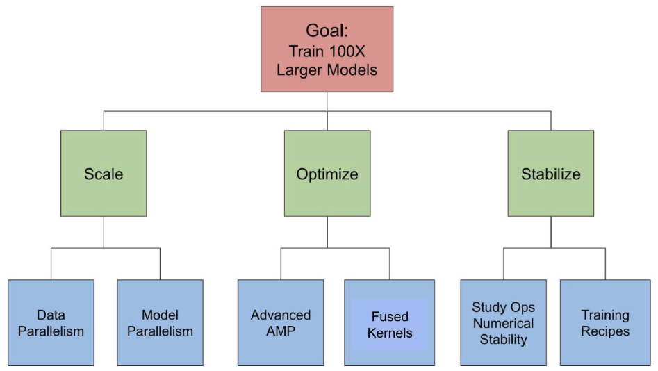
3.1 Addressing scaling challenges with data parallelism and model parallelism
We apply various forms of data and model parallelism to enable fitting very large models in GPU memory.
We use FairScale’s FullyShardedDataParallel (FSDP) API [4], based on PyTorch, to shard parameters, gradients, and optimizer state across multiple GPUs, thereby reducing the memory footprint per GPU. This process consists of the following three steps:
-
Step 1: We wrapped the entire model in a single FSDP instance. This shards the model parameters at the end of a forward pass and gathers parameters at the beginning of a forward pass. This enabled us to scale ~3x from 1.5B to 4.5B parameters.
-
Step 2: We experimented with wrapping individual model layers in separate FSDP instances. This nested wrapping further reduced the memory footprint by sharding and gathering parameters of individual model layers instead of an entire model. The peak memory is then determined by an individually wrapped transformer block in GPU memory in this mode instead of the entire model.
-
Step 3: We used activation-checkpoint to reduce the memory consumption by activations. It saves the input tensors and discards the intermediate activation tensors during the forward pass. These are recomputed during the backward pass.
In addition, we experimented with model-parallelism techniques such as pipeline parallelism [5], which allow us to scale to more GPUs without increasing the batch size.
3.2 Addressing optimization challenges with advanced AMP and kernel fusion
Advanced AMP
Automatic Mixed Precision (AMP) [6] training refers to training models using a lower precision of bits than FP32 or the default but still maintaining accuracy. We experimented with three levels of AMP as described below:
-
AMP O1: This refers to training in mixed precision where weights are in FP32 and some operations are in FP16. With AMP O1, the ops that might impact accuracy remain in FP32 and are not autocasted to FP16.
-
AMP O2: This refers to training in mixed precision but with more weights and ops in FP16 than in O1. Weights do not implicitly remain in FP32 and are cast to FP16. A copy of the master weights is maintained in the FP32 precision that is used by the optimizer. If we want the normalization layer weights in FP32 then we need to explicitly use layer wrapping to ensure that.
-
Full FP16: This refers to training in full FP16 where weights and operations are in FP16. FP16 is challenging to enable for training due to convergence issues.
We found that AMP O2 with LayerNorm wrapping in FP32 leads to the best performance without sacrificing accuracy.
Kernel Fusion
- To reduce GPU kernel launch overhead and increase GPU work granularity, we experimented with kernel fusions, including fused dropout and fused layer-norm, using the xformers library [7].
3.3 Addressing stability challenges by studying ops numerical stability and training recipes
BFloat16 in general but with LayerNorm in FP32
The bfloat16 (BF16) [8] floating-point format provides the same dynamic range as FP32 with a memory footprint identical to FP16. We found that we could train models in the BF16 format using the same set of hyperparameters as in FP32, without special parameter tuning. Nevertheless, we found that we need to keep LayerNorm in FP32 mode in order for the training to converge.
3.4 Final training recipe
A summary of the final training recipe.
- Wrap the outer model in an FSDP instance. Enable parameter sharding after the forward pass.
- Wrap individual ViT blocks with activation checkpointing, nested FSDP wrapping, and parameter flattening.
- Enable mixed precision mode (AMP O2) with bfloat16 representation. Maintain the optimizer state in FP32 precision to enhance numerical stability.
- Wrap normalization layers like LayerNorm in FP32 for better numerical stability.
- Maximize the Nvidia TensorCore utilization by keeping matrix dimensions to be multiple of 8. For More details check Nvidia Tensor Core Performance Guide.
4. Results
In this section, we show the scaling results of ViT on three types of tasks: (1) image classification, (2) object detection (3) video understanding. Our key result is that we are able to train massive ViT backbones across these vision tasks after applying the discussed scaling and optimization techniques. This enables vision research at a much larger scale. We trained the models to convergence to verify that we maintain the current baselines even with all the optimizations. A common trend in Figures 2, 3, 4 is that we are able to train up to 25B-param models with an epoch time of less than 4 hours on 128 A100 GPUs. The 60B and 120B models are relatively slower to train.
Figure 2 shows the image-classification scaling result. It plots the epoch time for training ViTs on ImageNet using 128 A100-80GB GPUs with different model sizes.
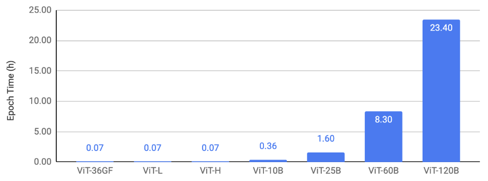
Figure 2: Image-classification scaling result.
Figure 3 shows the object-detection scaling result. It plots the epoch time for training ViTDet [9] with different ViT backbones on COCO using 128 A100-80GB GPUs.
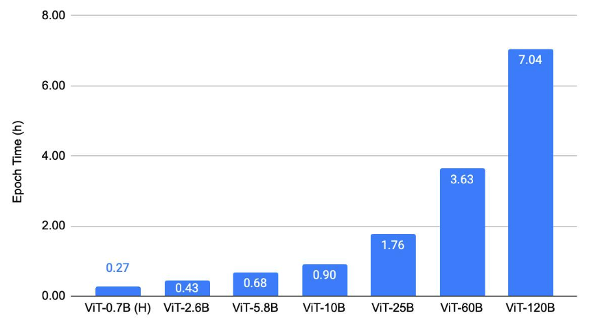
Figure 3: Object-detection scaling result.
Figure 4 shows the video-understanding scaling result. It plots the epoch time for training MViTv2 [10] models on Kinetics 400 [11] using 128 V100 (32 GB) GPUs in FP32.
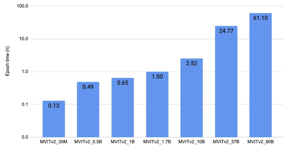
Figure 4: Video-understanding scaling result.
Figure 5 shows the optimization result with the ViT-H model in Figure 2 on 8 A100-40GB GPUs.
Three versions are used: (1) the baseline uses PyTorch’s DDP [12] with AMP O1, (2) FSDP + AMP-O2 + other optimizations, and (3) FSDP + FP16 + other optimizations. These optimizations altogether speed up the training by up to 2.2x.
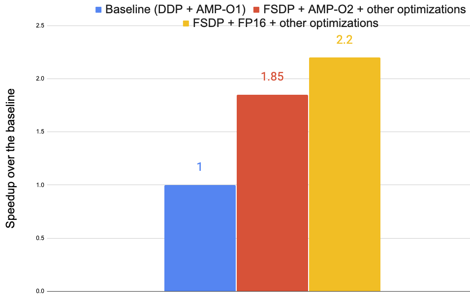
Figure 5: Training speedups from various optimizations.
5. Concluding Remarks
We have demonstrated the use of PyTorch with FairScale’s FullyShardedDataParallel (FSDP) API in writing large vision transformer models. We discuss our techniques for scaling and optimizing these models on a GPU cluster. We hope that this article can motivate others to develop large-scale ML models with PyTorch and its ecosystem.
