Speeding Up Reinforcement Learning with a New Physics Simulation Engine

Posted by C. Daniel Freeman, Senior Software Engineer and Erik Frey, Staff Software Engineer, Google Research

Reinforcement learning (RL) is a popular method for teaching robots to navigate and manipulate the physical world, which itself can be simplified and expressed as interactions between rigid bodies¹ (i.e., solid physical objects that do not deform when a force is applied to them). In order to facilitate the collection of training data in a practical amount of time, RL usually leverages simulation, where approximations of any number of complex objects are composed of many rigid bodies connected by joints and powered by actuators. But this poses a challenge: it frequently takes millions to billions of simulation frames for an RL agent to become proficient at even simple tasks, such as walking, using tools, or assembling toy blocks.

While progress has been made to improve training efficiency by recycling simulation frames, some RL tools instead sidestep this problem by distributing the generation of simulation frames across many simulators. These distributed simulation platforms yield impressive results that train very quickly, but they must run on compute clusters with thousands of CPUs or GPUs which are inaccessible to most researchers.

In “Brax – A Differentiable Physics Engine for Large Scale Rigid Body Simulation”, we present a new physics simulation engine that matches the performance of a large compute cluster with just a single TPU or GPU. The engine is designed to both efficiently run thousands of parallel physics simulations alongside a machine learning (ML) algorithm on a single accelerator and scale millions of simulations seamlessly across pods of interconnected accelerators. We’ve open sourced the engine along with reference RL algorithms and simulation environments that are all accessible via Colab. Using this new platform, we demonstrate 100-1000x faster training compared to a traditional workstation setup.

Three typical RL workflows. The left shows a typical workstation flow: on a single machine, with the environment on CPU, training takes hours or days. The middle shows a typical distributed simulation flow: training takes minutes by farming simulation out to thousands of machines. The right shows the Brax flow: learning and large batch simulation occur side by side on a single CPU/GPU chip.

Physics Simulation Engine Design Opportunities
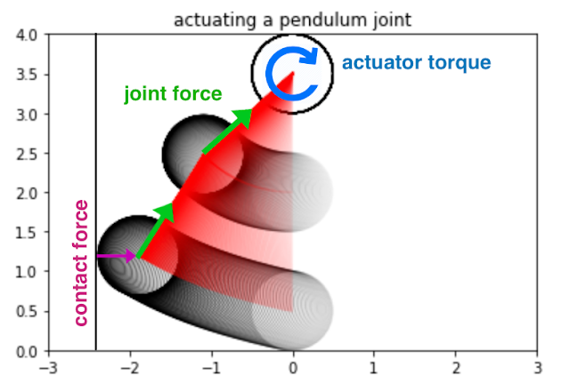
Rigid body physics are used in video games, robotics, molecular dynamics, biomechanics, graphics and animation, and other domains. In order to accurately model such systems, simulators integrate forces from gravity, motor actuation, joint constraints, object collisions, and others to simulate the motion of a physical system across time.

Simulation of three spherical bodies, a wall, two joints, and one actuator. For each simulation timestep, forces and torques are integrated together to update the positions, rotations, and velocities of each physical body.

Taking a closer look at how most physics simulation engines are designed today, there are a few large opportunities to improve efficiency. As we noted above, a typical robotics learning pipeline places a single learner in a tight feedback with many simulations in parallel, but upon analyzing this architecture, one finds that:

1. This layout imposes an enormous latency bottleneck. Because the data must travel over the network within a datacenter, the learner must wait for 10,000+ nanoseconds to fetch experience from the simulator. Were this experience instead already on the same device as the learner’s neural network, latency would drop to <1 nanosecond.
2. The computation necessary for training the agent (one simulation step, followed by one update of the agent’s neural network) is overshadowed by the computation spent packaging the data (i.e., marshalling data within the engine, then into a wire format such as protobuf, then into TCP buffers, and then undoing all these steps on the learner side).
3. The computations happening within each simulator are remarkably similar, but not exactly the same.

Brax Design
In response to these observations, Brax is designed so that its physics calculations are exactly the same across each of its thousands of parallel environments by ensuring that the simulation is free of branches (i.e., simulation “if” logic that diverges as a result of the environment state). An example of a branch in a physics engine is the application of a contact force between a ball and a wall: different code paths will execute depending on whether the ball is touching the wall. That is, if the ball contacts the wall, separate code for simulating the ball’s bounce off the wall will execute. Brax employs a mix of the following three strategies to avoid branching:

• Replace the discrete branching logic with a continuous function, such as approximating the ball-wall contact force using a signed distance function. This approach results in the most efficiency gains.
• Evaluate the branch during JAX’s just-in-time compile. Many branches based on static properties of the environment, such as whether it’s even possible for two objects to collide, may be evaluated prior to simulation time.
• Run both sides of the branch during simulation but then select only the required results. Because this executes some code that isn’t ultimately used, it wastes operations compared to the above.

Once the calculations are guaranteed to be exactly uniform, the entire training architecture can be reduced in complexity to be executed on a single TPU or GPU. Doing so removes the computational overhead and latency of cross-machine communication. In practice, these changes lower the cost of training by 100x-1000x for comparable workloads.

Brax Environments
Environments are tiny packaged worlds that define a task for an RL agent to learn. Environments contain not only the means to simulate a world, but also functions, such as how to observe the world and the definition of the goal in that world.

A few standard benchmark environments have emerged in recent years for testing new RL algorithms and for evaluating the impact of those algorithms using metrics commonly understood by research scientists. Brax includes four such ready-to-use environments that come from the popular OpenAI gym: Ant, HalfCheetah, Humanoid, and Reacher.

Brax also includes three novel environments: dexterous manipulation of an object (a popular challenge in robotics), generalized locomotion (an agent that goes to a target placed anywhere around it), and a simulation of an industrial robot arm.

Performance Benchmarks
The first step for analyzing Brax’s performance is to measure the speed at which it can simulate large batches of environments, because this is the critical bottleneck to overcome in order for the learner to consume enough experience to learn quickly.

These two graphs below show how many physics steps (updates to the state of the environment) Brax can produce as it is tasked with simulating more and more environments in parallel. The graph on the left shows that Brax scales the number of steps per second linearly with the number of parallel environments, only hitting memory bandwidth bottlenecks at 10,000 environments, which is not only enough for training single agents, but also suitable for training entire populations of agents. The graph on the right shows two things: first, that Brax performs well not only on TPU, but also on high-end GPUs (see the V100 and P100 curves), and second, that by leveraging JAX’s device parallelism primitives, Brax scales seamlessly across multiple devices, reaching hundreds of millions of physics steps per second (see the TPUv3 8×8 curve, which is 64 TPUv3 chips directly connected to each other over a high speed interconnect) .

Left: Scaling of the simulation steps per second for each Brax environment on a 4×2 TPU v3. Right: Scaling of the simulation steps per second for several accelerators on the Ant environment.

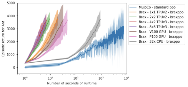
Another way to analyze Brax’s performance is to measure its impact on the time it takes to run a reinforcement learning experiment on a single workstation. Here we compare Brax training the popular Ant benchmark environment to its OpenAI counterpart, powered by the MuJoCo physics engine.

In the graph below, the blue line represents a standard workstation setup, where a learner runs on the GPU and the simulator runs on the CPU. We see that the time it takes to train an ant to run with reasonable proficiency (a score of 4000 on the y axis) drops from about 3 hours for the blue line, to about 10 seconds using Brax on accelerator hardware. It’s interesting to note that even on CPU alone (the grey line), Brax performs more than an order of magnitude faster, benefitting from learner and simulator both sitting in the same process.

Brax’s optimized PPO versus a standard GPU-backed PPO learning the MuJoCo-Ant-v2 environment, evaluated for 10 million steps. Note the x-axis is log-wallclock-time in seconds. Shaded region indicates lowest and highest performing seeds over 5 replicas, and solid line indicates mean.

Physics Fidelity
Designing a simulator that matches the behavior of the real world is a known hard problem that this work does not address. Nevertheless, it is useful to compare Brax to a reference simulator to ensure it is producing output that is at least as valid. In this case, we again compare Brax to MuJoCo, which is well-regarded for its simulation quality. We expect to see that, all else being equal, a policy has a similar reward trajectory whether trained in MuJoCo or Brax.

MuJoCo-Ant-v2 vs. Brax Ant, showing the number of environment steps plotted against the average episode score achieved for the environment. Both environments were trained with the same standard implementation of SAC. Shaded region indicates lowest and highest performing seeds over five runs, and solid line indicates the mean.

These curves show that as the reward rises at about the same rate for both simulators, both engines compute physics with a comparable level of complexity or difficulty to solve. And as both curves top out at about the same reward, we have confidence that the same general physical limits apply to agents operating to the best of their ability in either simulation.

We can also measure Brax’s ability to conserve linear momentum, angular momentum, and energy.

Linear momentum (left), angular momentum (middle), and energy (right) non-conservation scaling for Brax as well as several other physics engines. The y-axis indicates drift from the expected calculation (higher is smaller drift, which is better), and the x axis indicates the amount of time being simulated.

This measure of physics simulation quality was first proposed by the authors of MuJoCo as a way to understand how the simulation drifts off course as it is tasked with computing larger and larger time steps. Here, Brax performs similarly as its neighbors.

Conclusion
We invite researchers to perform a more qualitative measure of Brax’s physics fidelity by training their own policies in the Brax Training Colab. The learned trajectories are recognizably similar to those seen in OpenAI Gym.

Our work makes fast, scalable RL and robotics research much more accessible — what was formerly only possible via large compute clusters can now be run on workstations, or for free via hosted Google Colaboratory. Our Github repository includes not only the Brax simulation engine, but also a host of reference RL algorithms for fast training. We can’t wait to see what kind of new research Brax enables.

Acknowledgements
We’d like to thank our paper co-authors: Anton Raichuk, Sertan Girgin, Igor Mordatch, and Olivier Bachem. We also thank Erwin Coumans for advice on building physics engines, Blake Hechtman and James Bradbury for providing optimization help with JAX and XLA, and Luke Metz and Shane Gu for their advice. We’d also like to thank Vijay Sundaram, Wright Bagwell, Matt Leffler, Gavin Dodd, Brad Mckee, and Logan Olson, for helping to incubate this project.

¹ Due to the complexity of the real world, there is also ongoing research exploring the physics of deformable bodies. ^↩

Read More