Posted by Luiz GUStavo Martins, Developer Advocate
Transfer learning is a popular machine learning technique, in which you train a new model by reusing information learned by a previous model. Most common applications of transfer learning are for the vision domain, to train accurate image classifiers, or object detectors, using a small amount of data — or for text, where pre-trained text embeddings or language models like BERT are used to improve on natural language understanding tasks like sentiment analysis or question answering. In this article, you’ll learn how to use transfer learning for a new and important type of data: audio, to build a sound classifier.
There are many important use cases of audio classification, including to protect wildlife, to detect whales and even to fight against illegal deforestation.
With YAMNet, you can create a customized audio classifier in a few easy steps:
- Prepare and use a public audio dataset
- Extract the embeddings from the audio files using YAMNet
- Create a simple two layer classifier and train it.
- Save and test the final model
You can follow the code here in this tutorial.
The YAMNet model
YAMNet (“Yet another Audio Mobilenet Network”) is a pretrained model that predicts 521 audio events based on the AudioSet corpus.
This model is available on TensorFlow Hub including the TFLite and TF.js versions, for running the model on mobile and the web. The code can be found on their repository.
The model has 3 outputs:
- Class scores that you’d use for inference
- Embeddings, which are the important part for transfer learning
- Log Mel Spectrograms to provide a visualization of the input signal
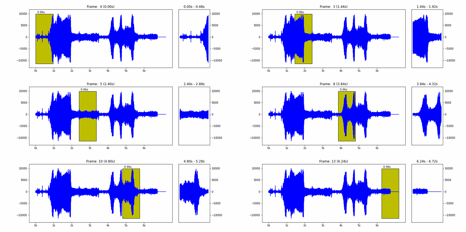
The model takes a waveform represented as 16 kHz samples in the range [-1.0, 1.0], frames it in windows of 0.96 seconds and hop of 0.48 seconds, and then runs the core of the model to extract the embeddings on a batch of these frames.
 |
| The 0.96 seconds windows hopping over a waveform |
As an example, trying the model with this audio file [link] will give you these results:
 |
| The first graph is the waveform. The second graph is the log-mel spectrogram. The third graph shows the class probability predictions per frame of audio, where darker is more likely. |
The ESC-50 dataset
To do transfer learning with the model, you’ll use the Dataset for Environmental Sound Classification, or ESC-50 for short. This is a collection of 2000 environmental audio recordings from 50 classes. Each recording is 5 seconds long and they came originally from the Freesound project.
The ESC-50 has the classes Dog and Cat that you’ll need.
The dataset has two important components: the audio files and a metadata csv file with the metadata about every audio file.
The columns in the metadata csv file contains information that will be used to train the model:
- Filename gives the name of the .wav audio file
- Category is the human-readable class name for the numeric target id
- Target is the unique numeric id of the category
- Fold ensures that clips originating from the same initial source are always contained in the same group. This is important to avoid cross-contamination when splitting the data into train, validation and test sets and for cross-validation.
For more detailed information you can read the original ESC paper.
Working with the dataset
To load the dataset, you’ll start from the metadata file and load it using the Pandas method read_csv.
With the loaded dataframe, the next steps are to filter by the classes that will be used, in this case: Dogs and Cats.
Next step would be to load the audio files to start the process but if there are too many audio files, just loading all of them to memory can be prohibitive and lead to out of memory issues. The best solution is to lazily load the audio files when needed. TensorFlow can help do this easily with tf.data.Dataset and the map method.
Let’s create the Dataset from the the previous created pandas dataframe and apply the load_wav method to all the files:
filenames = filtered_pd['filename']
targets = filtered_pd['target']
folds = filtered_pd['fold']

main_ds = tf.data.Dataset.from_tensor_slices((filenames, targets, folds))
main_ds = main_ds.map(load_wav_for_map)
Here, no audio file was loaded to memory yet since the mapping wasn’t evaluated. For example, if you request a size of the dataset for example (len(list(train_ds.as_numpy_iterator()))
), that would make the map function to be evaluated and load all the files.
The same technique will be used to extract all the features (embeddings) from each audio file.
Extracting the audio embeddings
Here you are going to load the YAMNet model from TensorFlow Hub. All you need is the model’s handle, and call the load method from the tensorflow_hub library.
yamnet_model_handle = 'https://tfhub.dev/google/yamnet/1'
yamnet_model = hub.load(yamnet_model_handle)
This will load the model to memory ready to be used.
For each audio file, you’ll extract the embeddings using the YAMNet model. For each audio file, YAMNet is executed. The embeddings output is paired with the same label and folder from the audio file.
def extract_embedding(wav_data, label, fold):
  ''' run YAMNet to extract embedding from the wav data '''
  scores, embeddings, spectrogram = yamnet_model(wav_data)
  num_embeddings = tf.shape(embeddings)[0]
  return (embeddings,
            tf.repeat(label, num_embeddings),
            tf.repeat(fold, num_embeddings))

main_ds = main_ds.map(extract_embedding).unbatch()
These embeddings will be the input for the classification model. From the model’s documentation, you can read that for a given audio file, it will frame the waveform into sliding windows of length 0.96 seconds and hop 0.48 seconds, and then run the core of the model. So, in summary, for each 0.48 seconds, the model will output one embedding array with 1024 float values. This part is also done using map(), so again, lazy evaluation and that’s why it executes so fast.
The final dataset contains the three used columns: embedding, label and fold.
The last dataset operation is to split into train, validation and test datasets. To do so the filter() method and use the fold field (an integer between 1 and 5) as criteria.
cached_ds = main_ds.cache()
train_ds = cached_ds.filter(lambda embedding, label, fold: fold < 4)
val_ds = cached_ds.filter(lambda embedding, label, fold: fold == 4)
test_ds = cached_ds.filter(lambda embedding, label, fold: fold == 5)
Training the Classifier
With the YAMNet embedding vectors and the label, the next step is to train a classifier that learns what’s a dog’s sound and what is a cat’s sound.
The classifier model is very simple with just two dense layers, but as you’ll see this is enough for the amount of data used.
my_model = tf.keras.Sequential([
    tf.keras.layers.Input(shape=(1024), dtype=tf.float32, name='input_embedding'),
    tf.keras.layers.Dense(512, activation='relu'),
    tf.keras.layers.Dense(len(my_classes))
])
Saving the final model
The model that was trained works and has good accuracy but the input it expects is not an audio waveform but an embedding array. To address this problem, the final model will combine YAMNet as the input layer and the model just trained. This way, the final model will accept a waveform and output the class:
input_segment = tf.keras.layers.Input(shape=(), dtype=tf.float32,
                                       name='audio')
embedding_extraction_layer = hub.KerasLayer('https://tfhub.dev/google/yamnet/1', trainable=False)
scores, embeddings, spectrogram = embedding_extraction_layer(input_segment)
serving_outputs = my_model(embeddings_output)
serving_outputs = ReduceMeanLayer(axis=0, name='classifier')(serving_outputs)
serving_model = tf.keras.Model(input_segment, serving_outputs)
serving_model.save(saved_model_path, include_optimizer=False)
To try the reloaded model, you can use the same way it was used earlier in the colab:
reloaded_model = tf.saved_model.load(saved_model_path)
reloaded_results = reloaded_model(testing_wav_data)
cat_or_dog = my_classes[tf.argmax(reloaded_results)]
This model can also be used with TensorFlow Serving with the ‘serving_default’
serving_results =  reloaded_model.signatures['serving_default'](testing_wav_data)
cat_or_dog = my_classes[tf.argmax(serving_results['classifier'])]
In this post, you learned how to use the YAMNet model for transfer learning to recognize audio of dogs and cats from the ESC-50 dataset.
Check out the YAMNet model on tfhub.dev and the tutorial on tensorflow.org. You can apply this technique to your own dataset, or to other classes in the ESC-50 dataset.
We would love to know what you can build with this! Share your project with us on social media by using the hashtag #TFHub.
Acknowledgements
We’d like to thank a number of colleagues for their contribution to this work: Dan Ellis, Manoj Plakal and Eduardo Fonseca for an amazing YAMNet model and support with the colab and multiple reviews.
Mark Daoust and Elizabeth Kemp have greatly improved the presentation of the material in this post and the associated tutorial.
